AutoEncoder based Collaborative Filtering

AutoRec

---

• 문제 의식
  • RBM-CF(Restricted Boltzmann Machines for Collaborative Filtering): 확률적 생성 모형으로서, 평점값마다 별도의 파라미터를 설정하므로 학습 파라미터 수가 급증하고, 확률 생성 과정을 근사 학습하므로 수렴 속도가 느림
  • LLORMA(Local Low-Rank Matrix Approximation): 행렬분해 기반 잠재요인 모형으로서, 사용자 취향이 전역적으로 일관되지 않을 수 있다는 전제 하에 사용자-아이템 상호작용 행렬을 다수의 하위 행렬로 재구성하고, 각각을 지역적 저차원(Local Low Rank)으로 근사하나, 구조가 복잡함
• AutoRec: 오토인코더 기반 협업필터링 모형으로서, 연속적 출력값을 결정론적 함수로 도출하는 단일 신경망 구조를 통해 선행 협업필터링 모형에 비해 계산 효율성과 구조적 간결성을 도모함
  • Sedhain, S., Menon, A. K., Sanner, S., & Xie, L.
    (2015, May).
    Autorec: Autoencoders meet collaborative filtering.
    In Proceedings of the 24th international conference on World Wide Web (pp. 111-112).

Notation

• $u=1,2,\cdots,M$: user idx
• $i=1,2,\cdots,N$: item idx
• $\mathbf{R} \in \mathbb{R}^{M \times N}$: user-item explicit feedback matrix
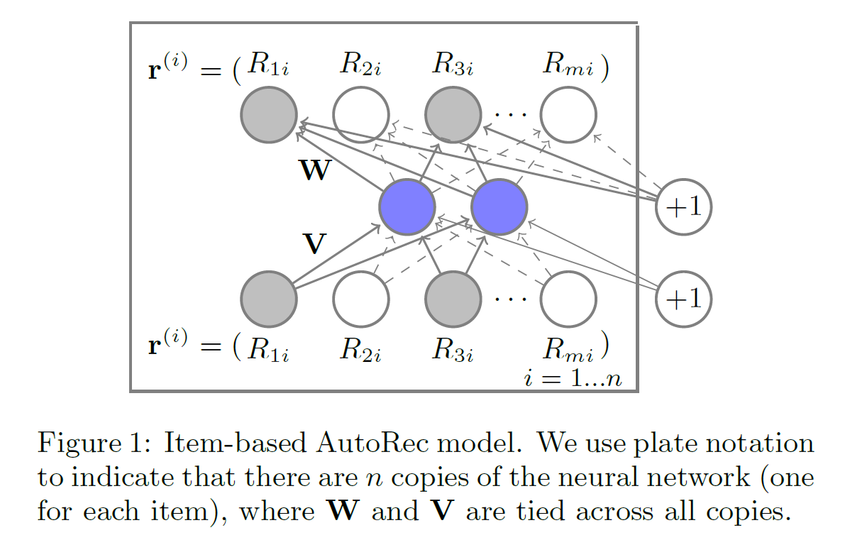
• $\mathbf{V} \in \mathbb{R}^{M \times K}$: linear transformation matrix @ encoder
• $\mathbf{W} \in \mathbb{R}^{K \times M}$: linear transformation matrix @ decoder
• $\overrightarrow{\beta} \in \mathbb{R}^{K}$: bias vector @ encoder
• $\overrightarrow{\mathbf{b}} \in \mathbb{R}^{M}$: bias vector @ decoder
• $f(\cdot)$: activation function @ encoder
• $g(\cdot)$: activation function @ decoder

How to Modeling

• Prediction

  \[\begin{aligned} \hat{\mathbf{r}}_{i} &= g\left[\mathbf{W} \cdot f(\mathbf{V} \cdot \overrightarrow{\mathbf{r}}_{i} + \overrightarrow{\beta}) + \overrightarrow{\mathbf{b}} \right] \end{aligned}\]

  • Encoder(Dimensionality Reduction):

    \[\begin{aligned} \overrightarrow{\mathbf{z}}_{i} &= f(\mathbf{V} \cdot \overrightarrow{\mathbf{r}}_{i} + \overrightarrow{\beta}) \end{aligned}\]

  • Decoder(Reconstruction):

    \[\begin{aligned} \hat{\mathbf{r}}_{i} &= g(\mathbf{W} \cdot \overrightarrow{\mathbf{z}}_{i} + \overrightarrow{\mathbf{b}}) \end{aligned}\]

• Optimization

  \[\begin{aligned} \hat{\Theta} &= \text{arg} \min{\sum_{i=1}^{N}{\Vert \overrightarrow{\mathbf{r}}_{i} - h(\overrightarrow{\mathbf{r}}_{i} ; \Theta) \Vert_{\mathcal{O}}^{2}} + \frac{\lambda}{2}\Vert \Theta \Vert_{F}^{2}} \end{aligned}\]
  • \(h(\overrightarrow{\mathbf{r}}_{i} ; \Theta)\): Reconstruction Output
  • \(\Theta\): Learning Parameters
  • \(\Vert \cdot \Vert_{\mathcal{O}}^{2}\): L2 Loss Computed only for Observed Entries
  • \(\Vert \cdot \Vert_{F}^{2}\): Regularization Term

CDAE

---

• 문제 의식: AutoRec 의 한계점
  • Implicit Feedback Problem
    • 구조적 편향 문제(Structural Bias): 관측과 미관측이 특정한 선택 경로와 제약 조건 하에서 발생했다는 점을 간과하고 선호와 비선호로 이분하는 데서 오는 체계적 왜곡
    • 자명해 문제(Trivial Solution): AutoRec 은 명시적 피드백 데이터 하에서 관측만을 사용하여 최적화를 수행하나, 암시적 피드백 데이터 하에서 이는 모든 상호작용을 $1$ 로 예측하는 자명해로 수렴함
  • Personalization Problem: AutoRec 은 행렬 복원에 초점을 맞추어 최적화를 수행하므로 히스토리는 유사하나 잠재적 선호 구조(latent preference structure)는 다른 사용자들 간에 제공되는 추천의 개인화가 미흡할 수 있음
• CDAE(Collaborative Denoising AutoEncoder): 잡음을 활용하여 암시적 피드백 데이터 하에서 손상된 선호도를 복원하고, 사용자 잠재 벡터를 활용하여 개인화 성능 향상을 꾀하는 오토인코더 기반 협업필터링 모형
  • Wu, Y., DuBois, C., Zheng, A. X., & Ester, M.
    (2016, February).
    Collaborative denoising auto-encoders for top-n recommender systems.
    In Proceedings of the ninth ACM international conference on web search and data mining (pp. 153-162).

Notation

• $u=1,2,\cdots,M$: user idx
• $i=1,2,\cdots,N$: item idx
• $\mathbf{Y} \in \mathbb{R}^{M \times N}$: user-item implicit feedback matrix
• $\mathbf{X} \in \mathbb{R}^{M \times N}$: masked $\mathbf{Y}$
• $\mathbf{M} \in \mathbb{R}^{M \times N}$: masking matrix
• $\overrightarrow{\mathbf{u}}_{u} \in \mathbb{R}^{K}$: user latent factor vector
• $\mathbf{V} \in \mathbb{R}^{M \times K}$: linear transformation matrix @ encoder
• $\mathbf{W} \in \mathbb{R}^{K \times M}$: linear transformation matrix @ decoder
• $\overrightarrow{\beta} \in \mathbb{R}^{K}$: bias vector @ encoder
• $\overrightarrow{\mathbf{b}} \in \mathbb{R}^{M}$: bias vector @ decoder
• $f(\cdot)$: activation function @ encoder
• $g(\cdot)$: activation function @ decoder

How to Modeling

• Generate Masking Noise

  \[\begin{aligned} \overrightarrow{\mathbf{x}}_{u} &= \overrightarrow{\mathbf{y}}_{u} \odot \overrightarrow{\mathbf{m}}_{u}, \quad \overrightarrow{\mathbf{m}}_{u} \sim \text{Bernouli}(1-p)^{N} \end{aligned}\]
  • \(\overrightarrow{\mathbf{m}}_{u} \sim \text{Bernouli}(1-p)^{N}\): \(m_{u,i} \sim \text{Bernouli}(1-p)\) independently

• Prediction

  \[\begin{aligned} \hat{\mathbf{y}}_{u} &= g\left[\mathbf{W} \cdot f(\mathbf{V} \cdot \overrightarrow{\mathbf{x}}_{u} + \overrightarrow{\mathbf{u}}_{u} + \overrightarrow{\beta}) + \overrightarrow{\mathbf{b}} \right] \end{aligned}\]

  • Encoder(Dimensionality Reduction):

    \[\begin{aligned} \overrightarrow{\mathbf{z}}_{u} &= f(\mathbf{V} \cdot \overrightarrow{\mathbf{x}}_{u} + \overrightarrow{\mathbf{u}}_{u} + \overrightarrow{\beta}) \end{aligned}\]

  • Decoder(Reconstruction):

    \[\begin{aligned} \hat{\mathbf{y}}_{u} &= g(\mathbf{W} \cdot \overrightarrow{\mathbf{z}}_{u} + \overrightarrow{\mathbf{b}}) \end{aligned}\]

• Optimization

  \[\begin{aligned} \Theta &= \text{arg} \min{\frac{1}{M}\sum_{u=1}^{M}{\mathbb{E}_{\mathbf{X} \sim P(\cdot \mid \mathbf{Y})}[\mathcal{L}(\mathbf{y}_{u}, \hat{\mathbf{y}}_{u})] + \frac{\lambda}{2} \Vert \Theta \Vert_{F}^{2}}} \end{aligned}\]
  • \(\mathcal{L}(\mathbf{y}_{u}, \hat{\mathbf{y}}_{u})\): Reconstruction Loss
  • \(\mathbb{E}_{\mathbf{X} \sim P(\cdot \mid \mathbf{Y})}\): Average Loss because of Stochasticity of Noise
  • \(\Theta\): Learning Parameters
  • \(\Vert \cdot \Vert_{F}^{2}\): Regularization Term

Mult-VAE

---

• 문제 의식
  • Implicit Feedback Problem
    • 구조적 편향 문제(Structural Bias): 관측을 선호, 미관측을 비선호로 확정적으로 간주하기에 불확실한 요소가 존재함(관측 불완전성)
    • 자명해 문제(Trivial Solution): 관측과 미관측의 비율이 균등하지 않아 모든 상호작용을 $0$ 으로 예측하는 자명해로 수렴할 위험이 있음(데이터 희소성)

  • Competitive Relationship between Items: 사용자 선택 과정에는 아이템 간 암묵적인 경쟁적 구조가 존재하므로 사용자가 특정 아이템과 상호작용할 확률은 다른 아이템과 상호작용할 확률과 독립적으로 계산되어서는 안 됨

  • Uncertainty of Latent Representation: 관측 불완전성, 데이터 희소성 등 암시적 피드백 데이터의 정보 불확실성으로 인하여 사용자 잠재 선호를 확정적으로 도출하기에 문제가 있으므로 사용자 선호가 취할 수 있는 다양한 가능성을 고려해야 함
• Mult-VAE(Multinomial Variational AutoEncoder): 확률적 생성 과정을 통해 표현의 다양성을 확보하되, 사전 정보로 규제함으로써 과잉 표현을 규제하고 일반화를 도모하는 오토인코더 기반 협업필터링 모형
  • Liang, D., Krishnan, R. G., Hoffman, M. D., & Jebara, T.
    (2018, April).
    Variational autoencoders for collaborative filtering.
    In Proceedings of the 2018 world wide web conference (pp. 689-698).

Notation

• $u=1,2,\cdots,M$: user idx
• $i=1,2,\cdots,N$: item idx
• $\mathbf{Y} \in \mathbb{R}^{M \times N}$: user-item implicit feedback matrix
• $f(\cdot)$: encoder networks
• $g(\cdot)$: decoder networks

How to Modeling

• Bayesian Framework

  • $Q$ is approx. dist. of latent preference vector:

    \[\begin{aligned} \overrightarrow{\mathbf{z}}_{u} \sim \mathcal{N}(\mu_{u}, \text{diag}(\sigma_{u}^{2})) \end{aligned}\]
    • $\mu_{u}, \text{diag}(\sigma_{u}^{2})$ is inferred by encoder networks $f(\cdot)$

  • $\Pi$ is prior dist. of latent preference vector:

    \[\begin{aligned} \overrightarrow{\mathbf{z}}_{u} \sim \mathcal{N}(0, \mathbf{I}) \end{aligned}\]

  • $P$ is likelihood:

    \[\begin{aligned} \overrightarrow{\mathbf{y}}_{u} \mid \overrightarrow{\mathbf{z}}_{u} \sim \text{Multinomial}(\vert \mathcal{R}_{u}^{+} \vert, \delta[g(\overrightarrow{\mathbf{z}}_{u})]) \end{aligned}\]
    • \(\overrightarrow{\mathbf{y}}_{u} \mid \overrightarrow{\mathbf{z}}_{u}\) is generated by decoder networks \(g(\cdot)\)
    • to reflect the competitive relationship between items when the user selects an item,
      • likelihood is multinomial dist., not $n$ independent binomial dist.
      • $\delta(\cdot)$ is softmax function, not sigmoid function

• Objective Function is ELBO:

  \[\begin{aligned} \hat{\Theta} &= \text{arg} \max{\mathbb{E}_{\mathbf{Z} \mid \mathbf{Y} \sim Q}[\log{p(\overrightarrow{\mathbf{y}}_{u} \mid \overrightarrow{\mathbf{z}}_{u})}] - \beta \cdot KL[Q(\overrightarrow{\mathbf{z}}_{u}) \Vert \Pi(\overrightarrow{\mathbf{z}}_{u})]} \end{aligned}\]