What? Bayesian
Based on the lecture “Bayesian Modeling (2024-1)” by Prof. Yeo Jin Chung, Dept. of AI, Big Data & Management, College of Business Administration, Kookmin Univ.
Bayesian Framework
Epistemology
-
인식론(Epistemology) : 믿음이 어떻게 정당화되어 앎이 되는가에 대한 철학적 논의
앎은 정당화된 참된 믿음(Knowledge is
JustifiedTrueBelief)- 믿음(Belief) : 해당 명제가 참임을 믿고 있다.
- 사실(Truth) : 해당 명제가 사실이어야 한다.
- 정당화(Justification) : 믿음에는 근거가 있어야 한다.
-
베이즈주의(Bayesianism) : 수량화된 인식론
확률적 귀납 개념에 따르면 과학 이론은 절대적 확실성을 가질 수 없지만 확실한 참과 확실한 거짓이라는 양극단 사이에 존재하는 인식적 값을 가질 수 있으며, 그 값은 새로운 증거에 의해 변경될 수 있다. (이영의, 2015, p.19)
- 형식 체계(Formalism) : 베이즈 정리(Bayes’ Theorem)
- 해석 체계(Interpretation) : 확률의 주관적 해석(Subjective interpretation)
-
베이지안 프레임워크(Bayesian Framework)
Formalism Bayes Module Interpretation \(p(\theta)\) 사전 확률 분포(Prior) 신념(Belief) \(p(\mathcal{D}\mid\theta)\) 우도(Likelihood) 참(Truth) \(p(\mathcal{D})\) 증거(Evidence) 근거(Reason) \(p(\theta\mid\mathcal{D})\) 사후 확률 분포(Posterior) 앎(Knowledge) \(p(\theta\mid\mathcal{D})=\displaystyle\frac{p(\mathcal{D}\mid\theta)p(\theta)}{p(\mathcal{D})}\) 베이즈 정리(Bayes’ Theorem) 정당화(Justification)
Formalism
-
콜모고로프의 확률 공리(Kolmogorov Probability Axiom)
확률 공간(Probability Space) $[\Omega, F, P]$ 는 다음을 이른다. 즉, $F$ 는 공집합이 아닌 집합 $\Omega$ 에 대하여 그 시그마 대수($\sigma$-Algebra)이다. 이때 확률함수(Probability Function) $P$ 는 $F$ 로부터 다음을 만족하는 실수로의 함수이다.
K1모든 $A \in F$ 에 대하여 $P(A) \ge 0$K2$P(\Omega)=1$K3$A \cap B = \emptyset$ 인 모든 $A,B \in F$ 에 대하여 $P(A \vee B) = P(A) + P(B)$
- 베이즈주의 확률 공리(Bayesian Probability Axiom)
B1$A,B \in S$ 에 대하여 $0 \le P(B \mid A) \le 1$B2$A$ 가 $B$ 를 논리적으로 함축하면 $P(B \mid A) = 1$B3$B,C$ 가 상호 배타적이면 $P(B \vee C\mid A) = P(B \mid A) + P(C \mid A)$B4$P(A) \ne 0$ 인 경우 $P(B \mid A) = \displaystyle\frac{P(A \wedge B)}{P(A)}$
- 성질(Property)
T1$B,C$ 가 독립적이면 $P(B \wedge C \mid A) = P(B \mid A) \cdot P(C \mid A)$T2$P(\neg B \mid A) = 1 - P(B \mid A)$T3$P(B \vee C \mid A) = P(B \mid A) + P(C \mid A) - P(B \wedge C \mid A)$T4$P(C \mid A) = P(B \mid A) \cdot P(C \mid A \wedge B) + P(\neg B \mid A) \cdot P(C \mid A \wedge \neg B)$
- 베이즈 정리(Bayes’ Theorem)
BT1$P(\theta), P(\mathcal{D}) > 0$ 이면 $P(\theta \mid \mathcal{D}) = \displaystyle\frac{P(\mathcal{D} \mid \theta) \cdot P(\theta)}{P(\mathcal{D})}$BT2$P(\theta_{1} \vee \cdots \vee \theta_{n})=1$ 이고 $\theta_{i} \vdash \neg \theta_{j}(i \ne j)$ 이면 $P(\theta_{k} \mid \mathcal{D}) = \displaystyle\frac{P(\mathcal{D} \mid \theta_{k}) \cdot P(\theta_{k})}{\sum_{i}{P(\mathcal{D} \mid \theta_{i}) \cdot P(\theta_{i})}}$BT3$P(\theta \mid \mathcal{D}) = \displaystyle\frac{P(\theta)}{P(\theta) + P(\mathcal{D} \mid \neg \theta) \cdot P(\neg \theta)/P(\mathcal{D} \mid \theta)}$
Interpretation
-
확률 해석(Probability Interpretation) : 확률함수 $P$ 의 의미를 규명하는 해석 체계
해석은 술어 논리, 리만 기하학, 양자역학과 같은 형식체계를 구성하는 공리들과 정의들에 등장하는 미정의된(Undefined) 또는 원초적(Primitive) 용어들에 일상적 의미를 부여하여 그런 공리들과 정리들이 준거 세계에 대해 참이 되도록 하는 작업을 의미한다. (이영의, 2015, p.19)
- 고전적 해석(Classical interpretation)
- 논리적 해석(Logical interpretation)
- 빈도적 해석(Frequentist interpretation)
- 성향적 해석(Propensity interpretation)
- 주관적 해석(Subjective interpretation)
-
주관적 해석(Subjective interpretation) (이영의, 2015, p.34)
베이즈주의는 이처럼 특정 진술에 대한 우리의 믿음, 즉 신념도에 양의 실수를 부여하는 것은 전형적인 확률 판단에 속한다고 보고, 그런 판단을 확률함수 $P$(Probability Function)로 표현한다. 확률함수 $P$ 는 특정 진술을 일정한 수치에 대응시킨다. (이영의, 2015, p.2)
s1확률은 특정 명제에 대한 행위자의 신념도이다.s2확률은 행위, 특히 내기 행위를 조사함으로써 가장 잘 확립될 수 있다.s3객관적인 확률은 없다. 만약 객관적 확률이 존재한다면 그것은 이차적 확률이다.s4사건은 고유한 확률을 갖지 않는다. 개인은 자신의 확률을 논리적으로 자유롭게 결정할 수 있다.s5합리적 개인의 신념은 확률론의 계산법과 무모순적이어야 하고, 동시에 그것에 의해 규제되어야 한다.
Condition
-
신념도를 확률로써 수량화할 수 있는가?
윤리적으로 중립인 명제에 대하여 그것의 참 여부에 따라 $0-1$ 사이의 서수적 효용을 획득하거나 상실할 수 있는 내기 상황을 가정함으로써, 베이즈주의는 개인의 신념도를 행위의 자발성과 동일시하는 행동주의적 접근을 취한다(이영의, 2015, p.35). 즉, 내기 상황 하에서 신념과 선호를 기대 효용의 형태로 연결하고, 이를 최적화 혹은 효용 극대화라는 선택으로써 측정 가능한 형태로 이끌어낸다. 또한 이 신념 체계의 정합성을 콕스 정리를 통해 형식적으로, 더치북 논증을 통해 실용적으로 입증한다.
Measurement Condition
-
측정 조건(Measurement Condition)
신념도는 측정될 방법을 규정할 수 있을 경우에만 완전한 의미를 가진다. (이영의, 2015, p.35)
-
램지 가정(Ramsey’s Assumption)
행위의 집합이 주어지면 합리적 행위자는 최대 기대값을 갖는 행위를 선택한다. (이영의, 2015, p.35)
-
기대 효용 이론(Expected Utility Theory)
$X$ 에 대한 행위자의 신념도가 $p$ 이라는 것은 그 행위자는 $X$ 이면 단위 $1$ 을 지불하고 그렇지 않은 경우에는 $0$ 을 지불하는 도박에 대해 $p$ 를 지불할 용의가 있다는 것이다. (de Finetti, 1937, p.62)
Consistency Condition
-
정합성 조건(Consistency Condition)
여러 가지 명제에 대한 개인의 신념도 집합은 일정한 방식으로 상호 간 일치하거나 입증되어야만 한다. (이영의, 2015, p.35)
-
베이즈주의 공준(Bayesianism Postulate)
이상적으로 합리적인 행위자의 신념도는 확률론의 공리체계를 준수한다. (이영의, 2015, p.19)
-
콕스 정리(Cox’s Theorem) | 논리적 정합화
함수 $G,H$ 가 실수 전체에 대하여 연속이고, 한 개인의 신념 함수 $b$ 가 논리 집합 $\mathcal{L}$ 에 대하여 $b:\mathcal{L} \times \mathcal{L} \to \mathbb{R}$ 인 단조 함수라고 하자. 아래 조건을 만족하는 신념 함수 $b$ 는 존재론적으로 유일한 확률 함수 $P$ 와 엄격히 증가하는 실수 함수 $F$ 에 대하여 $b(A \mid B) = F(P(A \mid B))$ 임을 만족한다. 즉, 신념 함수 $b$ 는 확률 함수 $P$ 와 동형이다.
-
논리 연산의 일관성(Associativity & Consistency) : 이변수 함수 $G$ 가 논리 연산 $\wedge$ 의 구조적 결합성과 일치하기 위해서는 형태가 곱셈형이거나 이와 동형이어야 함
\[\begin{aligned} b(A \wedge B \mid C) &= G(b(A \mid C), b(B \mid A \wedge C)) \end{aligned}\] -
부정의 일관성(Negation) : 일변수 함수 $H$ 가 부정을 나타내기 위해서는 확률의 여사건 법칙 $1-p$ 에 대응하는 형태를 만족해야 함
\[\begin{aligned} b(\neg A \mid B) &= H(b(A \mid B)) \end{aligned}\] -
존재 가능성(Non-Triviality) : 전적으로 확신하는 신념과 완전히 부정하는 신념은 서로 다른 값이어야 함
-
-
더치북 논증(Dutch Book Argument) | 실용적 정합화
특정인의 확률함수가 공리체계를 만족시키지 못할 경우에, 하나의 내기 전략이 있고 판돈의 집합이 있는 내기 상황에서 그는 결과에 상관없이 항상 일정한 액수를 잃게 된다. (이영의, 2015, p.58)
Epistemic Access to Truth
Constraining Priors
-
사전 확률 제약하기(Constraining Priors) : 베이즈주의적 합리성이 주관적 신념의 형식적 정합화를 넘어선 정당화를 제공하기 위해서는 사전 확률 분포가 논리적(Logical), 경험적(Empirical), 또는 규범적(Objective) 제약 하에 형성되어야 함
-
주관적 베이즈주의(Subjective Bayes) | Belief
나는 진심으로 그러한 절대적 의미에서의 모든 확률 개념을 반대한다. (중략) 확률은 우리가 그에 대해 정신적으로 또는 본능적으로 내리는 평가와 독립적으로 존재하지 않는다는 의미에서 “확률은 존재하지 않는다.” (de Finetti, 1977, p.199)
-
경험적 베이즈주의(Empirical Bayes) | Utility
그러므로 하나의 의견이 주어지면, 우리는 진위에 근거하여 그것을 칭찬하거나 책망할 수 있을 뿐이다. 특정한 형태의 습관이 주어지면 우리는 습관이 산출하는 신념도가 그것이 진리로 이끄는 실제 비율에 근접하거나 멀어지는가에 따라서 칭찬하거나 책망할 수 있다. 그렇다면 우리는 의견을 산출하는 습관들을 칭찬하거나 책망하는 것으로부터 파생적으로 의견들을 칭찬하거나 책망할 수 있다. (Ramsey, 1926, p.51)
-
객관적 베이즈주의(Objective Bayes) | Background, Non-Information
무차별의 원리가 주장하는 것은 만약 우리의 관심의 대상이 여러 가지 대안 중 어느 것보다 더 예측할 만한 어떠한 알려진 이유가 없다면 그러한 지식에 상대적으로 이러한 대안 각각에 대한 주장들은 동일한 확률을 갖는다는 점이다. (Keynes, 1921, p.42)
Washing Out Priors
-
베이즈주의가 주관적 신념을 넘어 인과 추론의 객관적 체계로서 정당화될 수 있는가?
절차의 합리성과 결과의 합리성이 대응하지 않을 경우는 어떻게 해야 하는가? (중략) 이 부분에서 우리의 논의에서 처음으로 합리성의 문제가 객관성의 문제와 관련된다. 진리성과 관련하여 어느 사회에서나 통용되는 기준들이 있으며 우리는 그것들이 객관적이라고 부른다. (중략) 베이즈주의적 객관성은 확실하지 않은 의견들 간 성립하는 간주관적 일치이다. (이영의, 2015, p.41)
-
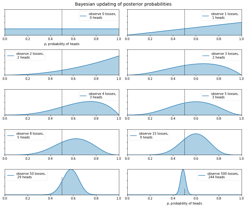
사전 확률 씻겨내기(Washing Out Priors) : 다양한 신념들은 충분한 근거가 주어지면 간주관적으로 수렴하며, 이 일치를 객관적 신념 상태로 해석할 수 있음
동전의 미래 행위에 대한 당신의 견해가 이웃 사람의 견해와 크게 다르더라도, 당신의 견해와 이웃 사람의 견해는 일상적으로 실험적인 던지기의 긴 연속에 베이즈의 정리를 적용하여 변형되어 거의 구별할 수 없게 될 것이다. (Edwards, Lindman, and Savage, 1963, p.197)
-
두브의 마틴게일 수렴 정리(Doob’s Martingale Convergence Theorem)
일반적 환경에서 조건화에 의한 확률 변화는 장기적으로 안정화된다. (이영의, 2015, p.54)
\(\mathbb{E}\left[\theta \mid \mathcal{D}_{n}\right] \to \mathbb{E}\left[\theta \mid \mathcal{D}_{\infty}\right]\)
Problem of Induction
-
귀납의 문제(Problem of Induction)
특정 사례들로부터 보편 결론을 이끌어낼 수 없다.
-
후험 일치성(Posterior Consistency)
확률 계산법을 준수하고 조건화 규칙에 따라 개정이 이루어진다면, 그리고 그러한 개정의 결과가 궁극적으로 참으로 수렴한다는 점이 보증된다면, 베이즈주의 추리에서는 귀납의 문제가 성립될 수 없다. (이영의, 2015, p.55)
-
슈바르츠 정리(Schwartz’s Theorem)
관측치 \(X \sim P(\theta)\), 모수 \(\theta \in \Theta\), 사전 확률 분포 \(\Pi\), 참 모수 \(\theta^{*}\) 에 대하여, \(\theta^{*}\) 의 근방에 위치한 \(\theta\) 가 사전 확률 분포에서 양의 질량을 가진다고 하자. 즉, \(\Pi\left(\{\theta : D_{KL}\left[P_{\theta^{*}} \Vert P_{\theta}\right] < \epsilon\}\right) > 0\) 이다. 이때 사후 확률 분포는 장기적으로 \(\theta^{*}\) 에 집중된다. 즉, \(\Pi\left(\theta^{*} \mid X_{1}, \cdots, X_{n}\right) \xrightarrow{n \to \infty} 1\) 이다.
-
조건화 규칙(Rule of Conditionalization)
-
엄밀조건화 규칙(Rule of Strict Conditionalization)
\[\begin{aligned} \pi\left(\theta\right) &= p\left(\theta \mid \mathcal{D}\right) \end{aligned}\] -
제프리 조건화 규칙(Jeffrey’s Conditionalization)
\[\begin{aligned} \pi\left(\theta\right) &= q\left(\mathcal{D}\right) \cdot p\left(\theta \mid \mathcal{D}\right) + q\left(\neg\mathcal{D}\right) \cdot p\left(\theta \mid \neg\mathcal{D}\right) \end{aligned}\]
-
Causal Inference
-
베이즈 정리가 인과 추론의 프레임워크로서 실제로 기능할 수 있는가?
\[\begin{aligned} P(\text{cause} \mid \text{outcome}) = \frac{P(\text{cause} \wedge \text{outcome})}{P(\text{outcome})} = \frac{P(\text{outcome} \mid \text{cause}) \cdot P(\text{cause})}{P(\text{outcome})} \end{aligned}\]어떤 알려지지 않은 사건($Z$)이 발생하고($p$) 실패한 횟수($n-p$)가 주어졌을 때, 하나의 시행에서 그 사건이 발생할 확률($\theta$)이 지정될 수 있는 두 가지 확률($\alpha, \beta$) 사이에 있을 기회가 요청된다($\alpha < \theta < \beta$). (Bayes, 1763, p.376)
베이즈 정리는 주어진 환경에서 하나의 사건($Z$)에 대해 동일한 환경에서 그것이 어떤 횟수만큼 발생했고($p$) 어떤 다른 횟수만큼 발생하는 데 실패했다는 것을($n-p$) 제외한 그 밖의 것에 대해 아무 것도 알지 못한다는 가정에서($\theta \sim \text{Uniform}$) 해당 사건이 발생할 확률($\theta$)을 판단할 방법을 찾는 일이다. (Price, 1763, 서문)
-
역추리 문제(Inverse Inference Problem) : 다양한 원인 중 하나로부터 발생했음이 틀림없는 한 가지 사건이 발생했다고 가정하고, 그 원인들이 존재할 각각의 확률을 추리하는 문제(이영의, 2015, p.62)
사건 $A,B$ 간에 선후관계가 존재한다고 가정하자. 즉, 사건 $A$ 는 사건 $B$ 에 선행한다. 이때 사건 $A,B$ 의 조건부 확률은 각각 다음을 나타낸다.
-
직접 확률(Direct Probability; $P(B \mid A)$) : 시행의 성질이 먼저 규정되고($P(A)$) 이어서 시행에서($P(B \mid A)$) 하나 또는 그 이상의 가능한 결과가 발생할 확률($P(A \wedge B)$) (이영의, 2015, p.62)
\[\begin{aligned} P(B \mid A) &= \frac{P(A \wedge B)}{P(A)} \end{aligned}\] -
역확률(Inverse Probability; $P(A \mid B)$) : 이미 시행의 결과가 제시되고($P(B)$) 그 다음 실제로 실행된 시행이($P(B \mid A)$) 가능한 시행 중($P(B)=\int{P(B \mid A) \cdot P(A)\text{d}A}$) 특정 시행에 해당할 확률($P(A \wedge B)$) (이영의, 2015, p.62)
\[\begin{aligned} P(A \mid B) &= \frac{P(A \wedge B)}{P(B)} \end{aligned}\]
-
-
당구대의 비유(Bayes’ Billiard Table Analogy)
당구대 $ABCD$ 를 가정하자. 공 $\mathcal{W}, \mathcal{O}$ 가 그 위에 굴려지면 어떤 하나의 동일한 부분에 정지할 동일한 확률을 가진다. $\mathcal{W}$ 으로 선분 $OS$ 의 위치가 결정된다. 그 우측 또는 좌측에 $\mathcal{O}$ 이 정지하는가에 따라서 사건 $Z$ 의 발생 또는 실패가 결정된다. $\mathcal{O}$ 를 연속하여 $n$ 회 던진 결과 $p$ 회만큼 우측에 정지했음이 관찰되었다. 이때 $AD$ 와 $OS$ 사이의 미지의 거리 $\theta$ 가 두 가지 값 $\alpha, \beta$ 사잇값을 취할 확률은?
-
공 $\mathcal{W}$ 가 던져지기 이전에 $\theta$ 가 $\alpha, \beta$ 사이에 있고, 사건 $Z$ 가 $n$ 번의 시행에서 $p$ 번 발생하고 $n-p$ 번 실패할 확률
\[\begin{aligned} P(\alpha < \theta < \beta, X=p) &= \int_{\alpha}^{\beta}{\binom{n}{p} \theta^{p}(1-\theta)^{n-p}\text{d}\theta} \end{aligned}\] -
사건 $Z$ 가 $p$ 번 발생할 확률
\[\begin{aligned} P(X=p) &= P(0 < \theta < 1, X=p)\\ &= \int_{0}^{1}{\binom{n}{p} \theta^{p}(1-\theta)^{n-p}\text{d}\theta} \end{aligned}\] -
$\theta$ 의 값에 대해 어느 것도 알려지기 이전에($0<\theta<1$), 사건 $Z$ 가 $n$ 번의 시행에서 $p$ 번 발생하고 $n-p$ 번 실패한 것으로 드러날 때, 그로부터 $\theta$ 가 $\alpha, \beta$ 사이에 있다고 추측한다면, 그 추측이 옳을 확률
\[\begin{aligned} P(\alpha < \theta < \beta \mid X=p) &= \frac{P(\alpha < \theta < \beta, X=p)}{P(0 < \theta < 1, X=p)}\\ &= \frac{\int_{\alpha}^{\beta}{\cancel{\binom{n}{p}} \theta^{p}(1-\theta)^{n-p}\text{d}\theta}}{\int_{0}^{1}{\cancel{\binom{n}{p}} \theta^{p}(1-\theta)^{n-p}\text{d}\theta}}\\ &= \frac{\int_{\alpha}^{\beta}{\theta^{p}(1-\theta)^{n-p}\text{d}\theta}}{\int_{0}^{1}{\theta^{p}(1-\theta)^{n-p}\text{d}\theta}} \end{aligned}\]
-
-
예증(Scholium)
내가 $Z$ 라고 불렀던 그러한 사건의 경우에, 일정 횟수로 시행하고($n$) 그것이 발생하고($p$) 실패한 횟수($n-p$)를 통해, 그것에 대해서는 다른 어떤 것도 알지 못한 상태에서 그것의 확률에 관해 추측할 수 있고(Non-Informative Prior of $\theta$), 언급한 면적들의 크기를 계산하는 일반적인 방법에 의해 그러한 추측이 옳을 기회를 알 수 있다(Posterior of $\theta \mid \mathcal{D}$).
그리고 동일한 규칙이 그것에 관해 이루어진 어떤 시행에서도, 우리가 사전에 전혀 알지 못하는 확률을 갖는 사건의 경우에도 사용될 수 있다는 것은 다음을 생각해보면 나타난 것 같다. 즉, 어떤 횟수의 시행에서 그것이 다른 횟수보다 어떤 가능한 다른 횟수로 발생할 것이라는 점을 생각할 이유가 없다.
그러므로 나는 다음부터 당연히 사건 $Z$ 에 대해 주어진 규칙($\theta$)이 또한 어떠한 시행이 이루어지거나 관찰되기 전에(Prior) 어떤 것도 알려지지 않은(Non-Informative) 사건의 확률(Posterior of $\theta \mid \mathcal{D}$)에도 이용될 수 있다고 간주할 것이다. 나는 그러한 사건을 알려지지 않은 사건(Non-Informative Prior)이라고 부를 것이다. (Bayes, 1763, p.393)
Reference
- 베이즈주의; 합리성으로부터 객관성으로의 여정
이영의. (2015). 한국연구재단 저술총서 4. 한국문화사