Decision Tree
Based on the lecture “Intro. to Machine Learning (2023-2)” by Prof. Je Hyuk Lee, Dept. of Data Science, The Grad. School, Kookmin Univ.

Decision Tree
-
결정 트리(Decision Tree): 순도(Uniformity)를 최대로 가져가는 이진 판별 규칙들로 구성된 수형도(Tree)를 세우고 관측치를 분류하는 알고리즘
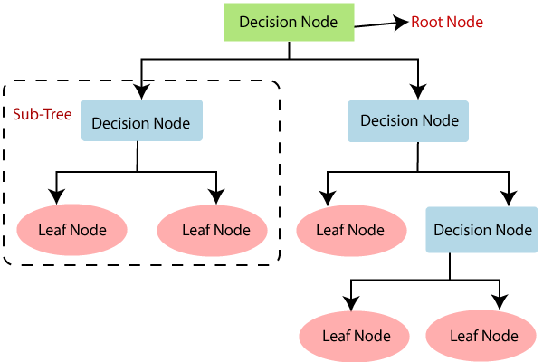
- 루트 노드(Root Node) : 깊이가 $0$ 인 꼭대기 노드로서 최상위 노드
- 결정 노드(Decision Node) : 규칙 조건
- 리프 노드(Leaf Node) : 하위 노드가 존재하지 않는 노드로서 최종 범주
- 서브트리(Subtree) : 어떠한 규칙 노드를 루트 노드로 가지는 하위 트리로서 판별 규칙 집합의 부분집합
Recursive Partitioning
-
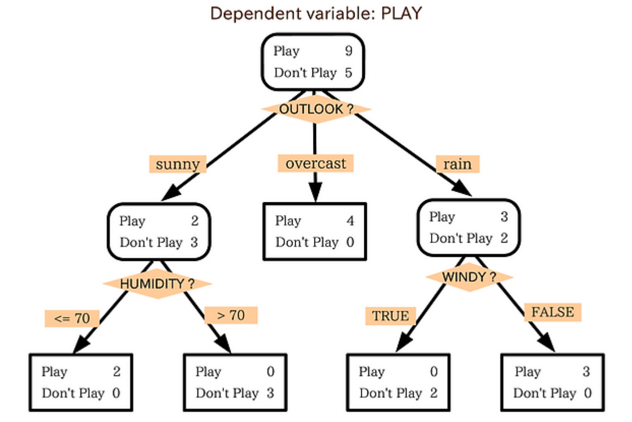
재귀적 분기(Recursive Partitioning) : 판별 규칙을 기준으로 상위 노드를 분할하여 순도가 높은 하위 노드를 생성하는 반복적인 과정
-
판별 규칙 : 어떤 분기에서 하나의 설명변수를 사용하여 생성한 분할 조건
-
순도(Purity) : 어떤 노드에 속한 관측치들이 동일한 범주에 속하는 정도
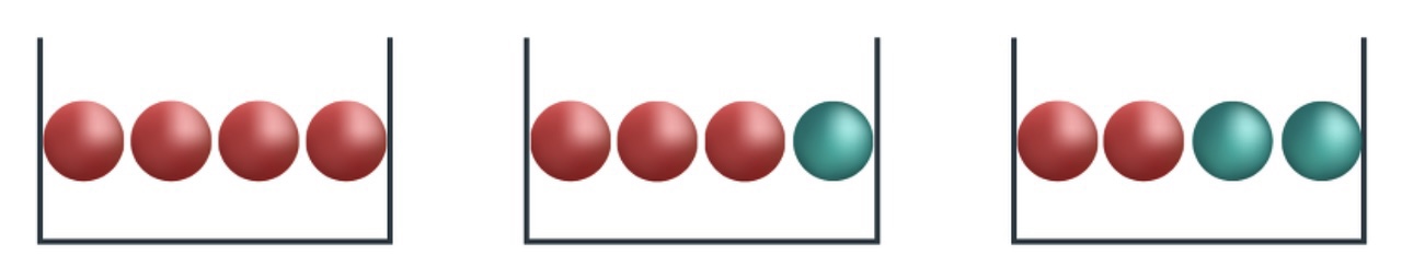
- 순도를 정확히 측정하기 어려우므로 그 대리변수로서 불순도(Impurity)를 사용함
-
Discriminant Rule
-
어떤 노드에 대하여, 설명변수 $X_{i} \ge x_{i}$ 를 기준으로 해당 노드를 분할한다고 하자
\[\begin{aligned} y=\begin{cases} N_{\text{Left}},\quad & \text{if} \quad X_{i} \ge x_{i}\\ N_{\text{Right}},\quad & \text{if} \quad X_{i} < x_{i}\\ \end{cases} \end{aligned}\] -
판별 규칙 $X_{i} \ge x_{i}$ 의 비용 $\mathcal{J}(X_{i} \ge x_{i})$ 는 다음과 같음
\[\begin{aligned} \mathcal{J}(X_{i} \ge x_{i}) &= \frac{m_{\text{Left}}}{m}I_{\text{Left}} + \frac{m_{\text{Right}}}{m}I_{\text{Right}} \end{aligned}\]- $m$ : 결정 노드에 속한 관측치 갯수
- $m_{\text{Left}}$ : 좌측 하위 노드로 분기한 관측치 갯수
- $I_{\text{Left}}$ : 좌측 하위 노드의 불순도
- $m_{\text{Right}}$ : 우측 하위 노드로 분기한 관측치 갯수
- $I_{\text{Right}}$ : 우측 하위 노드의 불순도
-
설명변수 $X_{i}$ 기준 분할 시 최적의 분기점 $\hat{x}_{i}$ 는 다음과 같음
\[\begin{aligned} \hat{x}_{i} =\text{arg} \min_{x_{i}}{\mathcal{J}(X_{i} \ge x_{i})} \end{aligned}\] -
특정 노드를 분할하는 최적의 설명변수 $\hat{X}_{i}$ 는 다음과 같음
\[\begin{aligned} \hat{X}_{i} = \text{arg} \min_{X_{i}}{\left\{\min{\mathcal{J}(X_{1})},\min{\mathcal{J}(X_{2})},\cdots,\min{\mathcal{J}(X_{n})}\right\}} \end{aligned}\]
Impurity
-
지니 지수(Gini Index) : 불순도를 경제적 불평등 개념 에 기초하여 계산한 지표
\[\begin{aligned} I(N_{k}) &= 1-\sum_{i=1}^{c}{p_{i}^2} \end{aligned}\]- $c$ : 범주 갯수
- $p_{i}$ : 노드 $N_{k}$ 에서 $i$ 번째 범주에 속하는 관측치 비율
-
엔트로피 지수(Entropy Index) : 불순도를 정보 획득의 불확실성 개념 에 기초하여 계산한 지표
\[\begin{aligned} I(N_{k}) &= -\sum_{i=1}^{c}{\left[p_{i} \cdot \log_{2}{p_{i}}\right]} \end{aligned}\]- $c$ : 범주 갯수
- $p_{i}$ : 노드 $N_{k}$ 에서 $i$ 번째 범주에 속하는 관측치 비율
Pruning
-
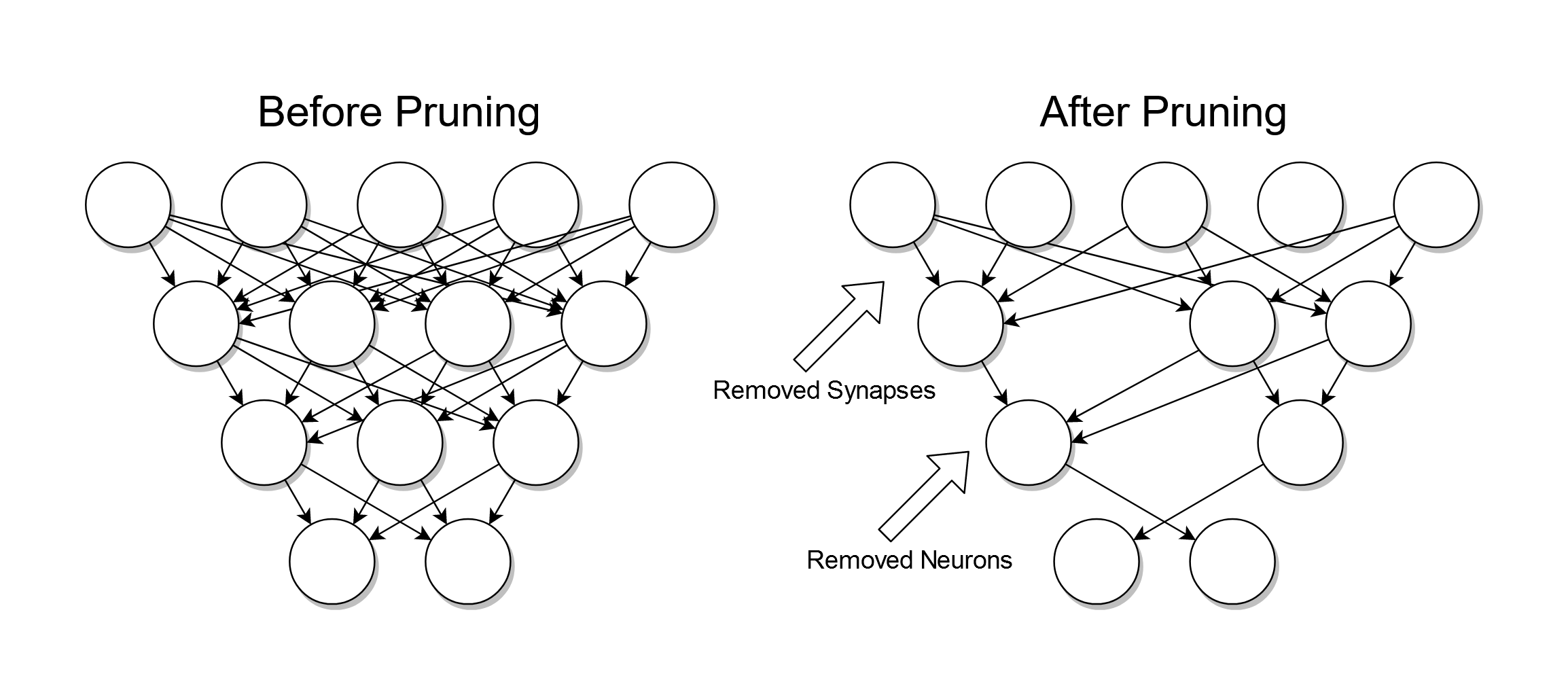
가지치기(Pruning) : 자세하게 구분된 영역을 통합함으로써 과적합을 방지하는 기법으로서, Full Tree 를 생성하여 모든 노드에 대하여 비용 복잡도 지수를 계산하고, 그 값이 가장 낮은 노드에 대하여 가지치기를 반복적으로 수행하면서 최적의 가지치기 강도 $\alpha$ 하 트리를 도출함
-
비용 복잡도 지수(Cost-Complexity)
\[\begin{aligned} R_{\alpha}(T) &= L(T) + \alpha \cdot \vert\text{Leaf}(T)\vert\\ L(T) &= \sum_{m=1}^{\vert\text{Leaf}(T)\vert}{\sum_{\mathbf{x}_{i} \in R_{m}}{\left(y_{i}-\hat{y}_{i}\right)^2}} \end{aligned}\]- $T$ : 타깃 노드를 루트 노드로 하는 서브트리
- $\text{Leaf}(T)$ : $T$ 의 리프 노드 집합
- $R_{m} \in \text{leaf}(T)$ : $T$ 의 $m$ 번째 리프 노드
- \(\mathbf{x}_{i} \in R_{m}\) : \(R_{m}\) 에 속한 \(i\) 번째 관측치 벡터
- $\alpha$ : 가지치기 강도
- $L(T)$ : $T$ 의 훈련 관측치에 대한 예측 손실
- $R_{\alpha}(T)$ : 타깃 노드의 비용 복잡도 지수
DTR
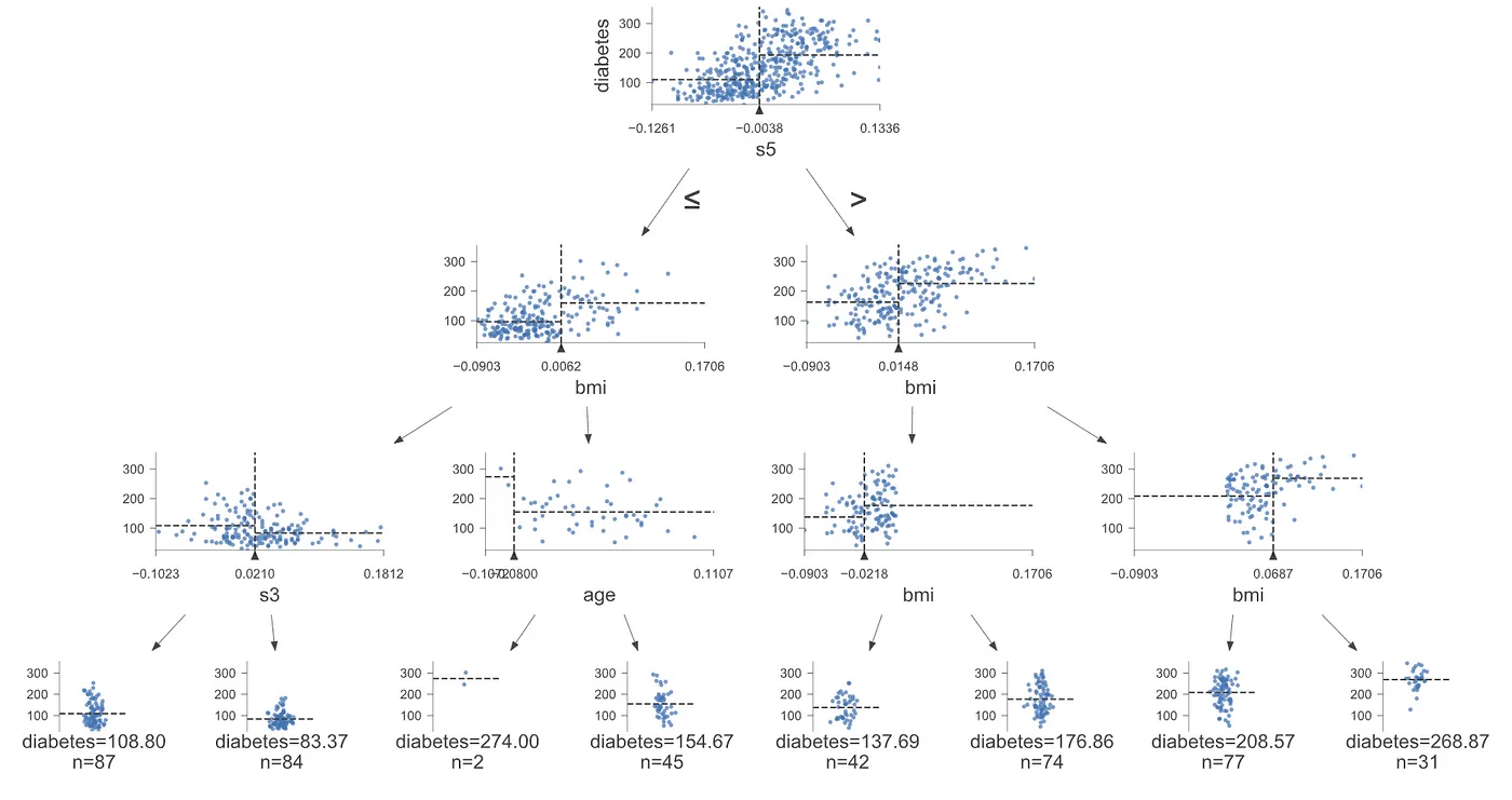
-
재귀적 분기
\[\begin{aligned} \hat{X}_{i} &= \text{arg} \min_{X_{i}}{\{\mathcal{J}(X_{1},\hat{x}_{1}),\mathcal{J}(X_{2},\hat{x}_{2}),\cdots,\mathcal{J}(X_{n},\hat{x}_{n})\}}\\ \hat{x}_{i} &= \text{arg} \min_{x_{i}}{\mathcal{J}(X_{i},x_{i})}\\ \mathcal{J}(X_{i},x_{i}) &= \frac{m_{\text{Left}}}{m}L_{\text{Left}}+\frac{m_{\text{Right}}}{m}L_{\text{Right}} \end{aligned}\] -
손실 함수
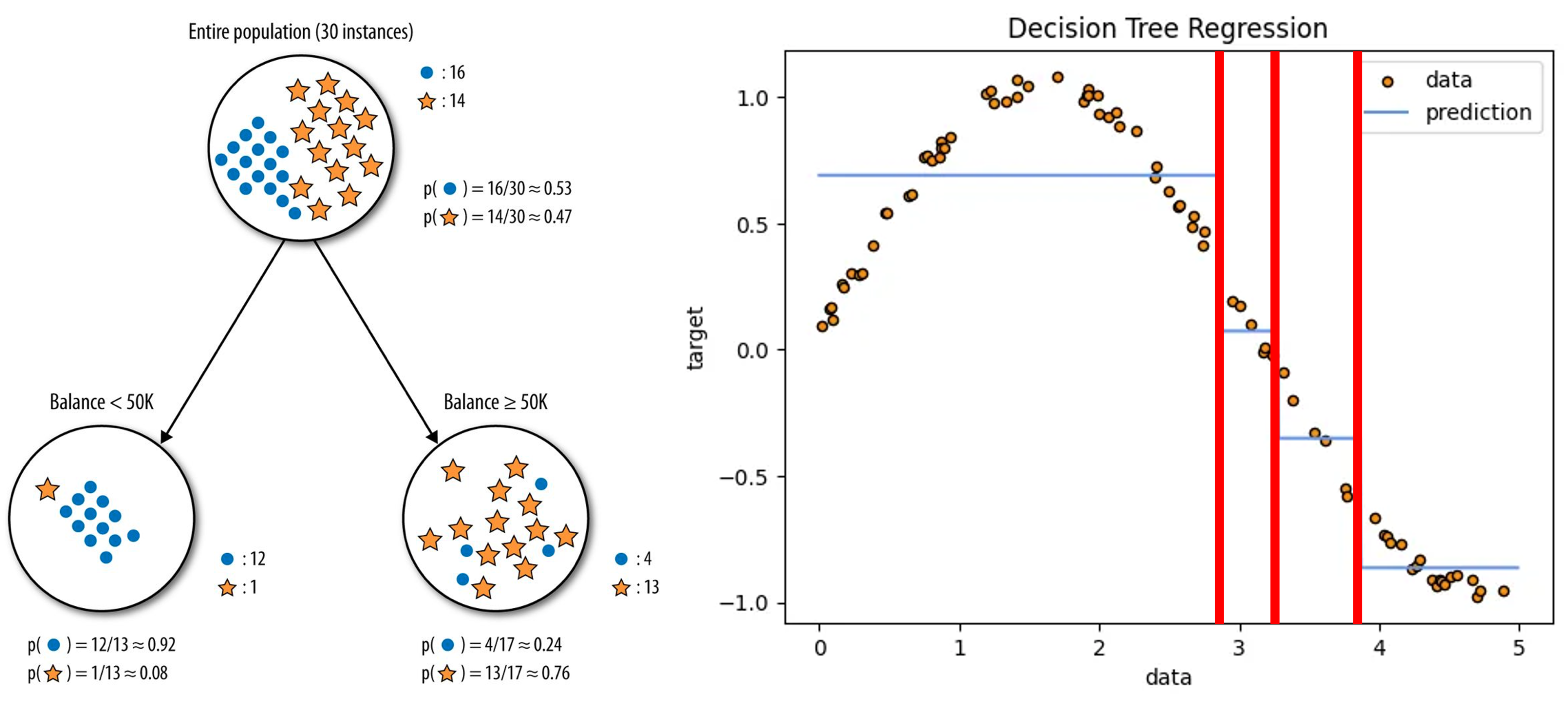
-
판별 분석 : 불순도(Impurity)를 최소화하도록 분기
\[\begin{aligned} \mathcal{L}_{\text{GINI}}(N_{k}) &= 1-\sum_{i=1}^{c}{p_{i}^2} \end{aligned}\] -
회귀 분석 : 오차(Error)를 최소화하도록 분기
\[\begin{aligned} \mathcal{L}_{\text{MSE}}(N_{k}) &= \sum_{i=1}^{m}{(y_{i}-\hat{y}_{i})^2} \end{aligned}\]
-