Ensemble
Based on the lecture “Intro. to Machine Learning (2023-2)” by Prof. Je Hyuk Lee, Dept. of Data Science, The Grad. School, Kookmin Univ.

Ensemble
-
앙상블 기법(Ensemble) : 예측 오차를 줄이기 위하여 다양한 모형들을 결합하는 기법
- 예측 오차를 어떻게 줄일 것인가?
- By Reducing Variance, Prevent Overfitting
- By Reducing Bias, Prevent Underfitting
- 모형 간 다양성을 어떻게 확보할 것인가?
- Provide different random subset of the training data to each other
- Using some measurement ensuring it is substantially different from the other members
- 모형별 결과물을 어떻게 결합할 것인가?
- Simple Voting
- Weighted Voting
Bias-Variance Trade-off
- Notation
- $Y$ : 실제 관측치
- $\varepsilon \sim N(0, \sigma^2)$ : 노이즈
- $f(X)$ : 실제 함수
- $\hat{f}(X)$ : $f(X)$ 에 대한 예측값
- $\overline{f}(X)$ : $\hat{f}(X)$ 의 평균
-
error segmentation:
\[\begin{aligned} \text{Error} &= \mathbb{E}\left[\left(Y-\hat{f}(X)\right)^{2}\right]\\ &= \mathbb{E}\left[\left(f(X) + \varepsilon - \hat{f}(X)\right)^{2}\right]\\ &= \mathbb{E}\left[\left(f(X)-\hat{f}(X)\right)^{2} + \varepsilon^{2} - 2 \cdot \varepsilon \cdot \left(f(X)-\hat{f}(X)\right) \right]\\ &= \mathbb{E}\left[\left(f(X)-\hat{f}(X)\right)^{2}\right] + \mathbb{E}\left[\varepsilon^{2}\right] - 2 \cdot \mathbb{E}\left[\varepsilon\right] \cdot \mathbb{E}\left[f(X)-\hat{f}(X) \right]\\ &= \mathbb{E}\left[\left(f(X)-\hat{f}(X)\right)^{2}\right] + \sigma^{2} \end{aligned}\] -
estimation error:
\[\begin{aligned} &\mathbb{E}\left[\left(f(X)-\hat{f}(X)\right)^{2}\right]\\ &= \mathbb{E}\left[\left(f(X)-\overline{f}(X)+\overline{f}(X)-\hat{f}(X)\right)^{2}\right]\\ &= \mathbb{E}\left[\left(f(X)-\overline{f}(X)\right)^{2}\right] + \mathbb{E}\left[\left(\overline{f}(X)-\hat{f}(X)\right)^{2}\right] + 2 \cdot \mathbb{E}\left[f(X)-\overline{f}(X)\right] \cdot \mathbb{E}\left[\overline{f}(X)-\hat{f}(X)\right]\\ &= \mathbb{E}\left[\left(f(X)-\overline{f}(X)\right)^{2}\right] + \mathbb{E}\left[\left(\overline{f}(X)-\hat{f}(X)\right)^{2}\right] \end{aligned}\] -
estimation error consists of bias and variance:
\[\begin{aligned} \mathrm{Bias}\left[\hat{f}(X)\right] &= \mathbb{E}\left[\hat{f}(X)\right] - f(X)\\ \mathrm{Var}\left[\hat{f}(X)\right] &= \mathbb{E}\left[\left(\overline{f}(X)-\hat{f}(X)\right)^{2}\right] \end{aligned}\] -
therefore:
\[\begin{aligned} \therefore \text{Error} &= \mathrm{Bias}^{2}\left[\hat{f}(X)\right] + \mathrm{Var}\left[\hat{f}(X)\right] + \sigma^{2} \end{aligned}\] -
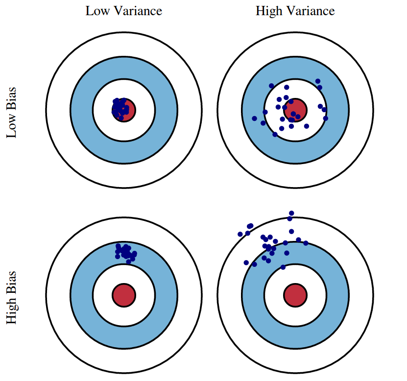
Bias-Variance Trade-off:
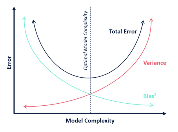
Biasis theunderfittingproblem that occurs when a model does not sufficiently learn the patterns of the training data.Varianceis theoverfittingproblem that occurs when a model adapts too much to the training data.
Why? Ensemble
\[\begin{aligned} \xi_{\text{ensemble}} \le \xi_{\text{avg}} \end{aligned}\]
-
$m$ 번째 모형의 예측값을 다음과 같이 정의하자
\[\begin{aligned} \underbrace{y_{m}(x)}_{\begin{array}{c} \text{predict value} \\ \text{of m-th model} \end{array}} &= \underbrace{f(x)}_{\text{real value}} + \underbrace{\epsilon_{m}(x)}_{\begin{array}{c} \text{error} \\ \text{of m-th model} \end{array}} \end{aligned}\] -
$m$ 번째 모형의 예측 오차의 자승을 다음과 같이 나타낼 수 있음
\[\begin{aligned} \therefore \mathbb{E}\left[\epsilon_{m}^{2}(x)\right] &= \mathbb{E}\left[\left(y_{m} - f(x)\right)^{2}\right] \end{aligned}\] -
개별 모형의 예측 오차 자승 평균 $\xi_{\text{avg}}$
\[\begin{aligned} \xi_{\text{avg}} &= \frac{1}{M}\sum_{m=1}^{M}{\mathbb{E}\left[\epsilon_{m}^{2}(x)\right]} \end{aligned}\] -
앙상블 모형의 예측 오차 자승 $\xi_{\text{ensemble}}$
\[\begin{aligned} \xi_{\text{ensemble}} &= \mathbb{E}\left[\left(\frac{1}{M}\sum_{m=1}^{M}{y_{m}(x)}-f(x)\right)^{2}\right]\\ &= \mathbb{E}\left[\left(\frac{1}{M}\sum_{m=1}^{M}{y_{m}(x)}-\frac{1}{M}\sum_{m=1}^{M}{f(x)}\right)^{2}\right]\\ &= \mathbb{E}\left[\left(\frac{1}{M}\sum_{m=1}^{M}{\epsilon_{m}(x)}\right)^{2}\right] \end{aligned}\] -
Cauchy-Schwartz Inequation
\[\begin{aligned} \left(\alpha_{1} \cdot \beta_{1} + \cdots + \alpha_{n} \cdot \beta_{n}\right)^{2} \le \left(\alpha_{1}^{2}+\cdots+\alpha_{n}^{2}\right)\left(\beta_{1}^{2}+\cdots+\beta_{n}^{2}\right) \end{aligned}\] -
$\text{if} \quad \alpha_{m}=1, \beta_{m}=\epsilon_{m}(x)$
\[\begin{aligned} \left(\sum_{m=1}^{M}{1 \cdot \epsilon_{m}(x)}\right)^{2} \le M \cdot \sum_{m=1}^{M}{\epsilon_{m}^{2}(x)} \end{aligned}\] -
$\times \displaystyle\frac{1}{M^{2}}$
\[\begin{aligned} \underbrace{\left(\frac{1}{M}\sum_{m=1}^{M}{\epsilon_{m}(x)}\right)^{2}}_{\xi_{\text{ensemble}}} \le \underbrace{\frac{1}{M} \sum_{m=1}^{M}{\epsilon_{m}^{2}(x)}}_{\xi_{\text{avg}}} \end{aligned}\]
Bagging
-
Bagging(
BootstrapAggregating) : 데이터 세트로부터 생성된 $M$ 개의 부트스트랩(Bootstrap)을 통해 $M$ 개의 개별 모형들을 병렬 학습하는 방법
\[\begin{aligned} y(x) &= \delta\Big[y_{1}(x), y_{2}(x), \cdots, y_{M}(x)\Big] \end{aligned}\]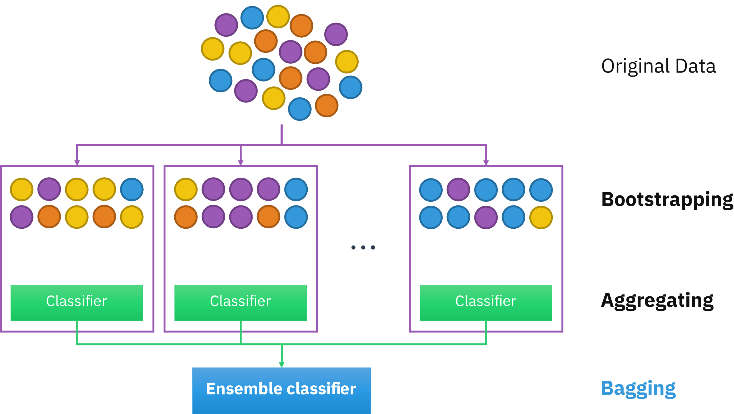
- By Reducing Variance, Prevent Overfitting
- Provide different random subset of the training data to each other
-
부트스트랩(Bootstrap) : 전체 데이터 세트를 $K$ 개의 데이터 블록으로 분할한 후 $K$ 번 복원추출하여 재구성한 훈련용 데이터 세트
-
데이터 세트 \(x \in \mathcal{D}\) 를 \(k\) 개의 데이터 블록 \(\Lambda^{(1)}, \cdots, \Lambda^{(K)}\) 으로 나누자
\[\begin{aligned} \mathcal{D} &= \left\{ x_{1}, x_{2}, \cdots, x_{N} \right\}\\ &= \Lambda^{(1)} \cup \Lambda^{(2)} \cup \cdots \cup \Lambda^{(K)} \quad \text{s.t.}\quad \Lambda^{(i)} \cap \Lambda^{(j \ne i)} = \emptyset \end{aligned}\] -
\(\Lambda^{(k)}\) 를 \(K\) 번 복원추출하여 \(m\) 번째 모형의 훈련용 데이터 세트를 구성함
\[\begin{aligned} \Omega^{(m)}_{\text{trn}} &= \left\{\Lambda^{(k)}_{l} \mid \Lambda^{(k)} \subseteq \mathcal{D}, k \in \{1, 2, \cdots, K\}, l=1,2,\cdots,K\right\} \end{aligned}\]
-
-
OOB(
OutofBag) : 부트스트랩에 포함되지 않는 데이터 블록 집합으로서 검증용 데이터 세트로 활용됨-
$m$ 번째 모형의 검증용 데이터 세트는 해당 모형의 부트스트랩에 포함되지 않은 데이터 블록으로 구성함
\[\begin{aligned} \Omega^{(m)}_{\text{val}} &= \bigcup_{k=1}^{K}{\Lambda^{(k)}} \setminus \Omega^{(m)}_{\text{trn}} \end{aligned}\] -
하나의 데이터 블록이 부트스트랩에 포함되지 않을 확률
\[\begin{aligned} \lim_{K \rightarrow \infty}{\left(1-\frac{1}{K}\right)^{K}} = e^{-1} \approx 0.368 \end{aligned}\]
-
-
Result Aggregating Function($\delta(\cdot)$)
- Simple Voting
- Weighted Voting(training accuarcy of individual models)
- Weighted Voting(probability result)
- Staking
Boosting
-
Boosting : 직렬로 나열된 개별 모형들에 대하여 모든 훈련 데이터 세트를 순차 학습하되, 현재 순번 모형이 오류를 줄이는 데 실패한 데이터 포인트에 대하여, 해당 포인트의 중요도를 가중함으로써 다음 모형이 더 집중하여 학습시키는 방법
\[\begin{aligned} y_{M}(x) &= \sum_{t=1}^{M}{\alpha_{t} \cdot h_{t}(x)} \end{aligned}\]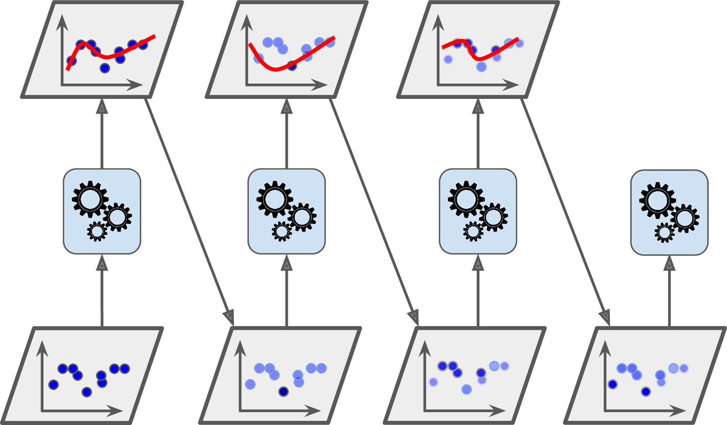
- By Reducing Bias, Prevent Underfitting
- Using some measurement ensuring it is substantially different from the other members
-
예측값 $y_{t}(x)$ 및 모형 $h_{t}(x)$
-
$t$ 번째 순번에서 $i$ 번째 관측치의 예측값 $y_{t}(x_{i})$ 을 다음과 같이 정의하자
\[\begin{aligned} \underbrace{y_{t}(x_{i})}_{\begin{array}{c} \text{predict value} \\ \text{of t-th model} \end{array}} &= \underbrace{f(x_{i})}_{\text{real value}} + \underbrace{\epsilon_{t}(x_{i})}_{\begin{array}{c} \text{error} \\ \text{of t-th model} \end{array}} \end{aligned}\] -
$t+1$ 번째 순번에서 $i$ 번째 관측치의 예측값 $y_{t+1}(x_{i})$ 을 다음의 규칙에 따라 갱신함
\[\begin{aligned} y_{t+1}(x_{i}) &= y_{t}(x_{i}) + \alpha_{t+1} \cdot h_{t+1}(x_{i}) \end{aligned}\] -
이때 $t+1$ 번째 순번 모형 $h_{t+1}$ 을 다음과 같이 도출함
\[\begin{aligned} h_{t+1} &= \text{arg} \min_{h}{\sum_{i=1}^{n}{L\left[\epsilon_{t}(x_{i}), h(x_{i})\right]}} \end{aligned}\]
-
-
모형별 중요도(가중 평균)
-
$t$ 번째 순번 모형의 중요도 $\alpha_{t}$ 를 다음과 같이 정의함
\[\begin{aligned} \alpha_{t} &= \frac{1}{2}\ln{\frac{1-\xi_{t}}{\xi_{t}}} \end{aligned}\] -
이때 $t$ 번째 순번 모형의 예측 오류율 $\xi_{t}$ 은 다음과 같음
\[\begin{aligned} \xi_{t} &= \frac{\sum_{i=1}^{n}{w_{i} \cdot \mathbb{I}\left[h_{t}(x_{i}) \ne f(x_{i})\right]}}{\sum_{j=1}^{n}{w_{j}}} \end{aligned}\]
-
-
관측치별 중요도
-
$t$ 번째 순번에서 $i$ 번째 관측치 $x_{i} \in \mathcal{D}$ 의 중요도 $P(x_{i})$ 를 다음과 같이 정의하자
\[\begin{aligned} P(x_{i}) &= \frac{w_{i}}{\sum_{j=1}^{n}{w_{j}}} \end{aligned}\] -
$i$ 번째 관측치 $x_{i} \in \mathcal{D}$ 의 가중치 $w_i$ 를 다음의 규칙에 따라 갱신함
\[\begin{aligned} w_i & \leftarrow w_{i} \cdot \exp{\bigg[\alpha_{t} \cdot \mathbb{I}\left[h_{t}(x_{i}) \ne f(x_{i})\right]\bigg]} \end{aligned}\]
-