Improvement of OLS

Bias-Variance Trade-off

---

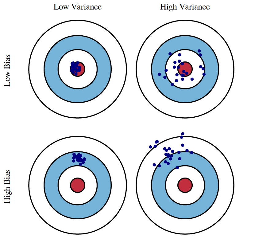
• Notation
  • $Y$ : 실제 관측치
  • $\varepsilon \sim N(0, \sigma^2)$ : 노이즈
  • $f(X)$ : 실제 함수
  • $\hat{f}(X)$ : $f(X)$ 에 대한 예측값
  • $\overline{f}(X)$ : $\hat{f}(X)$ 의 평균

• error segmentation:

  \[\begin{aligned} \text{Error} &= \mathbb{E}\left[\left(Y-\hat{f}(X)\right)^{2}\right]\\ &= \mathbb{E}\left[\left(f(X) + \varepsilon - \hat{f}(X)\right)^{2}\right]\\ &= \mathbb{E}\left[\left(f(X)-\hat{f}(X)\right)^{2} + \varepsilon^{2} - 2 \cdot \varepsilon \cdot \left(f(X)-\hat{f}(X)\right) \right]\\ &= \mathbb{E}\left[\left(f(X)-\hat{f}(X)\right)^{2}\right] + \mathbb{E}\left[\varepsilon^{2}\right] - 2 \cdot \mathbb{E}\left[\varepsilon\right] \cdot \mathbb{E}\left[f(X)-\hat{f}(X) \right]\\ &= \mathbb{E}\left[\left(f(X)-\hat{f}(X)\right)^{2}\right] + \sigma^{2} \end{aligned}\]

• estimation error:

  \[\begin{aligned} &\mathbb{E}\left[\left(f(X)-\hat{f}(X)\right)^{2}\right]\\ &= \mathbb{E}\left[\left(f(X)-\overline{f}(X)+\overline{f}(X)-\hat{f}(X)\right)^{2}\right]\\ &= \mathbb{E}\left[\left(f(X)-\overline{f}(X)\right)^{2}\right] + \mathbb{E}\left[\left(\overline{f}(X)-\hat{f}(X)\right)^{2}\right] + 2 \cdot \mathbb{E}\left[f(X)-\overline{f}(X)\right] \cdot \mathbb{E}\left[\overline{f}(X)-\hat{f}(X)\right]\\ &= \mathbb{E}\left[\left(f(X)-\overline{f}(X)\right)^{2}\right] + \mathbb{E}\left[\left(\overline{f}(X)-\hat{f}(X)\right)^{2}\right] \end{aligned}\]

• estimation error consists of bias and variance:

  \[\begin{aligned} \mathbb{Bias}\left[\hat{f}(X)\right] &= \mathbb{E}\left[\hat{f}(X)\right] - f(X)\\ \mathbb{Var}\left[\hat{f}(X)\right] &= \mathbb{E}\left[\left(\overline{f}(X)-\hat{f}(X)\right)^{2}\right] \end{aligned}\]

• therefore:

  \[\begin{aligned} \therefore \text{Error} &= \mathbb{Bias}^{2}\left[\hat{f}(X)\right] + \mathbb{Var}\left[\hat{f}(X)\right] + \sigma^{2} \end{aligned}\]

• Bias-Variance Trade-off:

  

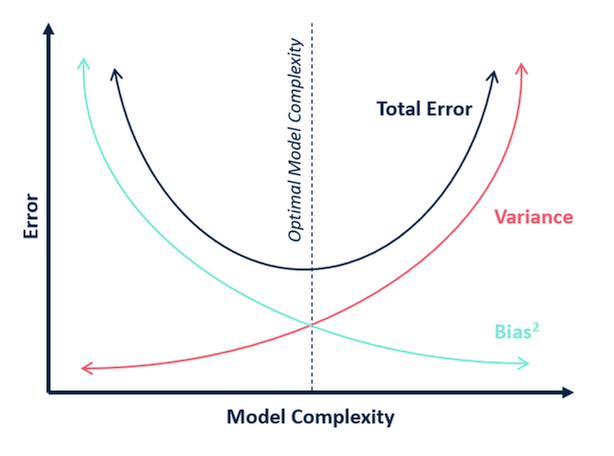
  • Bias is the underfitting problem that occurs when a model does not sufficiently learn the patterns of the training data.
  • Variance is the overfitting problem that occurs when a model adapts too much to the training data.

Improvement of OLS

---

최소자승추정량은 BLUE(Best Linear Unbias Estimator)로서, 편향이 $0$ 인 추정량 중 분산이 가장 작은 추정량임. 만약 편향이 $0$ 이어야 한다는 제약 조건을 완화한다면 분산을 더 줄일 수 있지 않을까?

• 변수 선택(Feature Selection) : $p$ 개의 설명변수 중 반응변수와 관련이 있다고 생각되는 설명변수들을 식별하여 추정하는 방법
  • 전진 선택(Forward Selection)
  • 후진 선택(Backward Elimination)
  • 혼합 선택(Stepwise Selection)
• 수축(Shrinkage) : $p$ 개의 설명변수를 모두 포함하는 모형을 추정하되, 회귀계수를 최소자승추정량보다 작은 값으로 수축함으로써 분산을 줄이는 방법
  • Ridge Regression
  • LASSO Regression
• 차원축소(Dimension Reduction) : $p$ 개의 설명변수를 저차원 공간으로 사영(Projection)하는 방법
  • 주성분 분석(Principal Component Analysis; PCA)
  • 선형 판별 분석(Linear Discriminant Analysis; LDA)

Feature Selection

---

Occam’s Razor

Entities should not be multiplied beyond necessity.

• 전진 선택(Forward Selection) : 어떤 변수도 선택되지 않은 상태에서 가장 설명력이 좋은 변수를 하나씩 추가하는 방법

  \[\begin{aligned} \hat{x}_{i}&=\text{arg} \max_{x_{i}}R^2[y,f(x_{i})]\\ \hat{x}_{j}&=\text{arg} \max_{x_{j}}R^2[y,f(x_{j \ne i};\hat{x}_{i})]\\ \hat{x}_{k}&=\text{arg} \max_{x_{k}}R^2[y,f(x_{k \ne i,j};\hat{x}_{i},\hat{x}_{j})]\\ &\vdots \end{aligned}\]

• 후진 선택(Backward Elimination) : 모든 변수가 포함된 상태에서 시작하여 불필요한 변수를 하나씩 제거하는 방법

  \[\begin{aligned} \hat{x}_{i}&=\text{arg} \max_{x_{i}}R^2[y,f(\not{x_{i}})]\\ \hat{x}_{j}&=\text{arg} \max_{x_{j}}R^2[y,f(\not{x_{j \ne i}};\not{\hat{x}_{i}})]\\ \hat{x}_{k}&=\text{arg} \max_{x_{k}}R^2[y,f(\not{x_{k \ne i,j}};\not{\hat{x}_{i}},\not{\hat{x}_{j}})]\\ &\vdots \end{aligned}\]

• 혼합 선택(Stepwise Selection) : 어떤 변수도 선택되지 않은 상태에서 Forward Selection 과 Backward Elimination 을 번갈아 수행하는 방법

Metrics

• Adjusted Coefficient of Determination($\text{Adj.}R^2$)

  \[\text{Adj.}R^2 = \frac{(n-1)R^2-p}{n-p-1}\]

• Akaike Information Criteria(AIC)

  \[\begin{aligned} \text{AIC} &= -2\ln{\hat{L}}+2k \end{aligned}\]

  • $\hat{L}$ : 모델 적합도로서 \(\mathbf{x}_{i}\) 가 주어졌을 때 $y_{i}$ 가 발생할 가능성

    \[\begin{aligned} \hat{L} &= \prod_{i=1}^{n}{P(Y=y^{(i)} \mid X=\mathbf{x}^{(i)};\hat{\mathbf{b}})}\\ \hat{\mathbf{b}} &= \begin{pmatrix}\hat{\beta_{0}}&\hat{\beta_{1}}&\cdots&\hat{\beta_{d}}\end{pmatrix} \end{aligned}\]

  • $k$ : 모델 복잡도

• Bayesian Information Criteria(BIC)

  \[\begin{aligned} \text{BIC} &= -2\ln{\hat{L}}+k\ln{n} \end{aligned}\]

Shrinkage Methods

---

• p-norm : $n$ 차원 벡터 $\mathbf{x}=\begin{pmatrix}x_{1}&x_{2}&\cdots&x_{n}\end{pmatrix}$ 의 크기를 정의하는 방법

  

  \[\Vert x \Vert _{p}=(\vert x_{1} \vert ^{p}+ \vert x_{2} \vert ^{p}+\cdots+ \vert x_{n} \vert ^{p})^{\frac{1}{p}}\]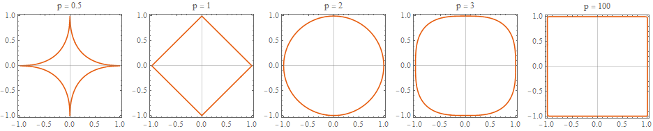

• 가중치 규제(Weight Regulation) : 회귀계수 최적값을 탐색함에 있어 회귀계수 벡터 $\beta$ 의 크기에 제약을 두는 것

  

  \[\begin{aligned} \hat{\beta} &= \text{arg} \min_{\beta}{\left[L_{OLS}+\lambda \Vert \beta \Vert _{p}^{2}\right]} \end{aligned}\]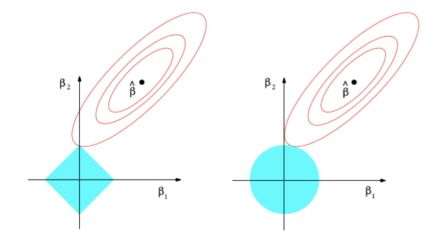
  • $L_{OLS}(\beta)$ : 최소자승법에 기초한 손실 함수
  • $\beta$ : 회귀계수 벡터
  • $\lambda$ : 회귀계수 벡터 $\beta$ 크기 제약 강도
  • p=1 : LASSO
  • p=2 : Ridge

---

Sourse

• http://scott.fortmann-roe.com/docs/BiasVariance.html
• https://github.com/lovit/python_ml_intro
• https://ekamperi.github.io/machine%20learning/2019/10/19/norms-in-machine-learning.html
• https://observablehq.com/@petulla/l1-l2l_1-l_2l1-l2-norm-geometric-interpretation