Markov Chain Monte Carlo
Based on the lecture “Bayesian Modeling (2024-1)” by Prof. Yeo Jin Chung, Dept. of AI, Big Data & Management, College of Business Administration, Kookmin Univ.

Markov Chain Monte Carlo
-
마르코프 체인 몬테 카를로(
MarkovChainMonteCarlo) : 이전 단계에서 추출한 표본을 기반으로 다음 단계의 표본을 순차로 추출하여 사후 분포에 근사하는 방법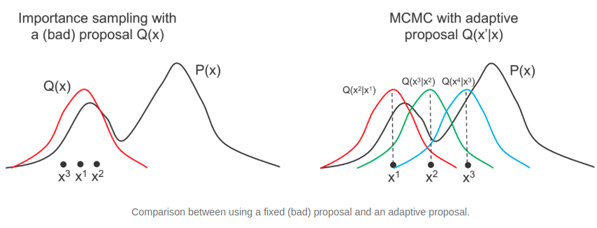
- Random-walk based MCMC
- Metropolis algorithm
- Metropolis–Hastings
- Random-Walk Metropolis
- Independence sampler
- Gibbs Sampling based MCMC
- Full Gibbs sampler
- Blocked Gibbs
- Collapsed Gibbs
- Gradient based MCMC
- Hamiltonian Monte Carlo
- No-U-Turn Sampler
- Riemannian Manifold HMC
Metropolis Hastings Method
-
메트로폴리스 헤이스팅스 방법(Metropolis Hastings Method) : 목표 분포의 산 모양을 추정하기 위하여, 확률 밀도가 높은 지역일수록(봉우리가 높은 지역일수록) 그 근방에서 더 많은 조약돌을 모으는 방법
-
inital sample:
\[\theta^{(t=0)}\] -
sampling candidate state $\psi$:
\[\psi \sim \mathcal{N}(\theta^{(t)},\sigma^2)\] -
conditional acceptance:
\[\theta^{(t+1)} =\begin{cases}\begin{aligned} \psi, \quad &\text{if} \quad u<\alpha(\theta^{(t)},\psi) \quad \text{for} \quad u \sim \text{Uniform}(0,1)\\ \theta^{(t)}, \quad &\text{otherwise} \end{aligned}\end{cases}\]
-
-
목표 분포(Target Dist.) : 파라미터 $\theta^{(t)}$ 의 사후 확률 분포
\[p(\theta^{(t)}\mid \mathcal{D}) \propto p(\theta^{(t)}) \cdot p(\mathcal{D} \mid \theta^{(t)})\] -
제안 분포(Proposal Dist.) : 시점 $t$ 에서 수락된 파라미터 샘플 $\theta^{(t)}$ 에 기반하여 다음 시점 $t+1$ 에서 샘플링 위치 $\psi$ 를 제안하는 분포
\[q(\psi \mid \theta^{(t)}) = \mathcal{N}(\theta^{(t)},\sigma^2)\]-
제안 분포가 $\theta^{(t)}$ 을 중심으로 하는 종형 분포인 경우:
\[q(\psi \mid \theta^{(t)}) = q(\theta^{(t)} \mid \psi)\] -
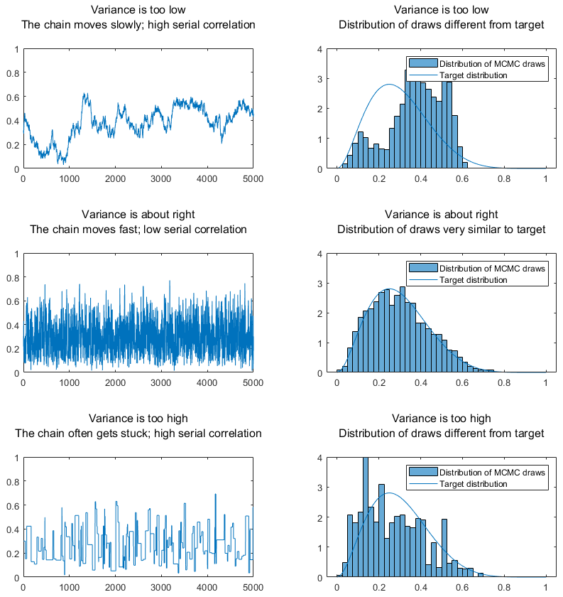
$\sigma^2$ 의 크기와 샘플링 수렴 여부의 관계:
-
-
수락 확률(Acceptance Prob.) : $\psi$ 를 다음 시점의 샘플 $\theta^{(t+1)}$ 로 수락할 확률
\[\begin{aligned} \alpha(\theta^{(t)}, \psi) &= \min{\left[1, \frac{p(\psi \mid \mathcal{D})}{p(\theta^{(t)} \mid \mathcal{D})} \cdot \frac{q(\theta^{(t)} \mid \psi)}{q(\psi \mid \theta^{(t)})}\right]}\\ &= \min{\left[1, \frac{p(\psi \mid \mathcal{D})}{p(\theta^{(t)} \mid \mathcal{D})}\right]} \quad \text{s.t.} \quad \psi \sim \mathcal{N}(\theta^{(t)},\sigma^2)\\ &\propto \min{\left[1, \frac{p(\psi) \cdot p(\mathcal{D} \mid \psi)}{p(\theta^{(t)}) \cdot p(\mathcal{D} \mid \theta^{(t)})}\right]} \end{aligned}\]
Auto-Correlation
-
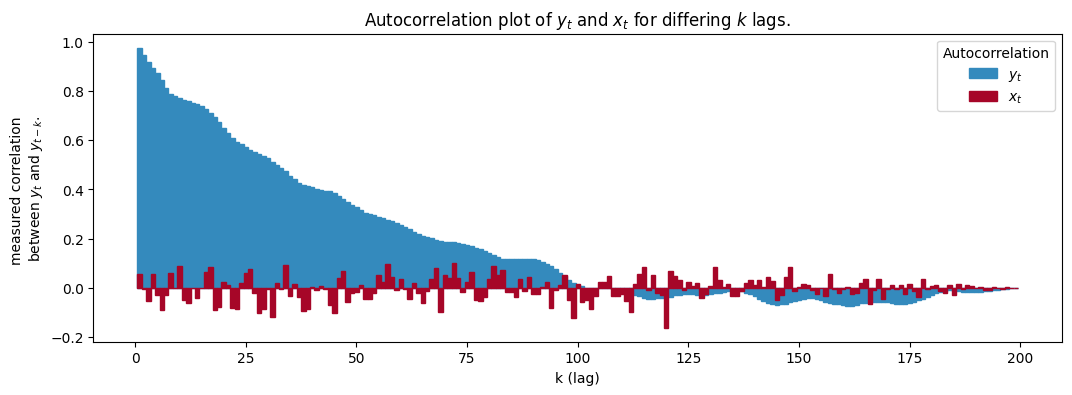
자기상관(Auto-Correlation) : 순차로 발생한 일련의 관측치 ${x^{(t)} \mid t\text{ is time point}}$ 간에 존재하는 상관관계
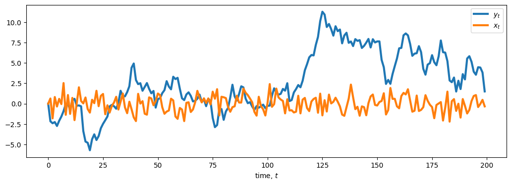
- $x^{(t)} \sim N(0,1) \quad \text{for} \quad x^{(0)} = 0$
- $y^{(t)} \sim N(y^{(t-1)},1) \quad \text{for} \quad y^{(0)} = 0$
-
자기상관계수(Auto-Correlation Coefficient) : 순서에 의미가 있는 데이터에서, 현재 시점의 값 $x^{(t)}$ 과 그 과거 또는 미래의 값 $x^{(t-k)}$ 간의 상관관계를 측정하는 지표
\[R(k)=\text{Corr}(x^{(t)},x^{(t-k)})\]-
$k$ : 시간 간격(Lag)
-
-
솎아내기(Thinning) : 매 $k$ 번째 표본을 선택함으로써 자기상관을 줄이는 방법
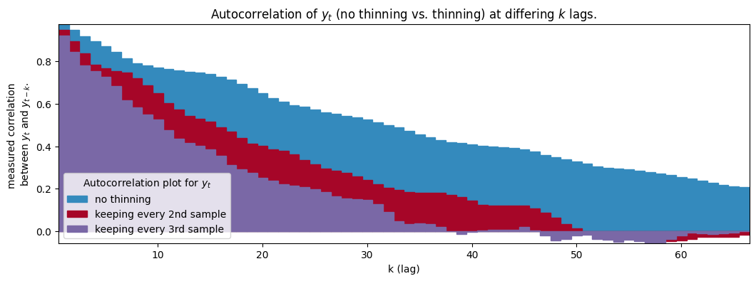
- 통상 $k \le 10$ 으로 설정함
-
선행 구간(Burn-in Period) : 수렴 상태에 도달하기 전, 초기값 $x^{(t=0)}$ 의 영향력을 최소화하기 위해 일부 반복을 무시하는 구간

PyMC Summary Indicator
-
Posterior Mean: 사후 평균 추정치
\[\hat{\mu}=\frac{1}{N}\sum_{i=1}^{N}{\theta_{i}}\] -
Posterior Standard Deviation: 사후 평균 추정치의 표준편차
\[\hat{\sigma}=\sqrt{\frac{1}{N-1}\sum_{i=1}^{N}{(\theta_{i}-\hat{\mu})^{2}}}\] -
\[\mathrm{MCSE}_{\mathrm{mean}} =\sqrt{\mathrm{Var}(\hat{\mu})}\approx \frac{\hat{\sigma}}{\sqrt{\mathrm{ESS}}}\]MonteCarloStandardError: 사후 평균 추정치의 몬테카를로 표준오차- Mean: 사후 분포의 중심 위치 추정 불확실성으로서 중심 위치 추정의 안정성
- Std: 사후 분포의 폭 추정 불확실성으로서 신뢰구간 추정의 정확성
-
\[\mathrm{ESS}=\frac{MN}{1+2\sum_{t=1}^{\infty}{\rho_{t}}}\]EffectiveSampleSize: 샘플 간 자기상관을 보정한 독립 샘플 수- Bulk: 중심부에서의 표본 독립성으로서 사후 분포의 중심 위치 통계량의 신뢰도
- Tail: 꼬리부에서의 표본 독립성으로서 신뢰구간 경계의 신뢰도
-
Gelman–Rubin Statistic (Potential Scale Reduction Factor): 체인 간 수렴성 평가 지표
\[\hat{R}=\sqrt{\frac{B}{W}}\]-
Definition:
\[\begin{aligned} \bar{\theta}^{(k)}:=\frac{1}{N}\sum_{i=1}^{N}{\theta_{i}^{(k)}}, \quad \bar{\theta}:=\frac{1}{M}\sum_{k=1}^{M}{\bar{\theta}_{k}} \end{aligned}\] -
Between-chain variance:
\[\begin{aligned} B=\frac{N}{M-1}\sum_{k=1}^{M}{(\bar{\theta}^{(k)} - \bar{\theta})^{2}} \end{aligned}\] -
Within-chain variance:
\[\begin{aligned} W&=\frac{1}{M}\sum_{k=1}^{M}{s_{k}^{2}}\\ s_{k}^{2}&=\frac{1}{N-1}\sum_{i=1}^{N}{(\theta_{i}^{(k)}-\bar{\theta}^{(k)})^{2}} \end{aligned}\]
-
Source
- https://www.statlect.com/fundamentals-of-statistics/Markov-Chain-Monte-Carlo