BNNs (2) Monte Carlo Dropout
Gal, Y., & Ghahramani, Z. (2016, June). Dropout as a bayesian approximation: Representing model uncertainty in deep learning. In international conference on machine learning (pp. 1050-1059). PMLR.

Monte Carlo Dropout
- 불확실성(Uncertainty): 어떠한 사건에 대하여 확신할 수 없는 상태
-
우발적 불확실성(Aleatoric Uncertainty): 관측치에 내재된 잡음 혹은 무작위성으로 인해 발생하는 불확실성
-
인식적 불확실성(Epistemic Uncertainty): 정보 부족으로 인해 발생하는 불확실성
- 모형의 불확실성(Model Uncertainty): 관측치 부족, 모형 가정 부적합 등으로 인하여 모형이 메커니즘을 제대로 모사하지 못하는 문제
- 표현의 불확실성(Latent Uncertainty): 다대일 대응 구조로 인하여 치역만으로 정의역을 유일하게 식별할 수 없는 구조적 비식별성 문제
- 메커니즘의 불확실성(Mechanistic Uncertainty): 모형이 모사하고자 하는 실제 메커니즘이 확정적으로 규명될 수 없는 문제
-
-
문제 의식
-
모형의 불확실성(Model Uncertainty):
인공신경망 알고리즘은 파라미터 수가 매우 많아 과적합 문제(Overfitting) 에서 자유롭지 못함. 여기서 과적합이란, 모형의 복잡도가 데이터 셋이 제공하는 정보량보다 심화되어 발생하는 현상임. 이는 정보가 부족한 상황에서 단일 가설을 확신하여 예측하는 과신의 문제(Overconfidence) 에서 비롯함.
-
계산 복잡도(Computational Cost):
과신의 문제를 직접 다루는 베이즈 추론을 신경망에 적용하는 경우 계산 복잡도 문제에서 자유로울 수 없음. 가령 Bayes by Backprop 의 경우 파라미터마다 평균과 분산을 각각 계산해야 하므로 추론해야 하는 파라미터 수가 결정론적 신경망의 두 배가 됨.
-
-
MC Dropout(Monte-Carlo Dropout): 드롭아웃이 적용된 인공신경망의 가우시안 프로세스의 유한 차원 근사임을 증명하여 결정론적 신경망과 동일한 비용으로 불확실성 모델링이 가능함을 확인함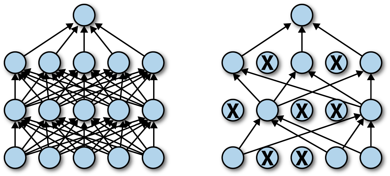
1 layer nn analysis
-
1 layer nn:
\[\begin{aligned} f(x) &:=\frac{1}{\sqrt{N}}\sum_{i=1}^{N}{w_{i}\sigma(v_{i}x)} \end{aligned}\]- $v_{i}$: input -> hidden weight
- $\sigma$: activation function
- $w_{i}$: hidden -> output weight
- $N$: num of node unit
-
therefore 1 layer nn can be considered as an element on the function space consisting of a basis function, $\phi_{i}(x):=\sigma(v_{i}x)$.
\[\begin{aligned} f(\cdot)\in\mathcal{F}:=\mathrm{span}\{\phi_{1}(\cdot),\phi_{2}(\cdot),\cdots,\phi_{N}(\cdot)\} \end{aligned}\] -
apply dropout mask $m_{i}$ to weight $w_{i}$:
\[\begin{aligned} \beta_{i} &=w_{i} \cdot m_{i} \quad m_{i}\sim\mathrm{Bernoulli}(p)\\ &=\begin{cases}w_{i},\quad &p\\0,\quad &1-p\end{cases} \end{aligned}\] -
since the function value $f(x)$ is a sum of random features $\beta_{i}\phi_{i}(x)$, $\beta_{i}\phi_{i}(x)$, it becomes a random variable.
\[\begin{aligned} \therefore f(x) &=\frac{1}{\sqrt{N}}\sum_{i=1}^{N}{\beta_{i}\phi_{i}(x)} \end{aligned}\]
Lindeberg-Feller CLT
-
Lindeberg-Feller CLT:
합계 변수 $f:=\sum_{i=1}^{N}{X_{i}}$ 에 대하여 (1) 개별 변수 $X_{i}$ 가 상호 독립이고($X_{i}\perp X_{j}$), (2) 개별 변수 $X_{i}$ 의 분산이 유한하며($\mathrm{Var}\left[X_{i}\right]<\infty$), (3) 합계 변수 $f$ 의 분산이 유한하다면($\mathrm{Var}\left[f\right]<\infty$), 합계 변수 $f$ 의 분포는 $N\to\infty$ 일 때 $X_{i}$ 의 분포와 상관없이 가우시안 분포에 근사한다($f\sim\mathcal{N}$).
-
independence condition:
\[\beta_{i}\phi_{i}(x) \perp \beta_{j}\phi_{j}(x)\]- $v_{i}\perp v_{j}$ (input weight)
- $w_{i}\perp w_{j}$ (output weight)
- $m_{i}\perp m_{j}$ (dropout weight)
-
finiteness of individual variance:
\[\begin{aligned} \mathrm{Var}\left[\frac{1}{\sqrt{N}}\beta_{i}\phi_{i}(x)\right] &= \frac{1}{N}\phi_{i}^{2}(x)\cdot w_{i}^{2}\cdot p(1-p) < \infty \end{aligned}\] -
finite convergence of total variance:
\[\begin{aligned} \lim_{N\to\infty}{\mathrm{Var}\left[f(x)\right]} &=\lim_{N\to\infty}{\frac{1}{N}\sum_{i=1}^{N}{\phi_{i}^{2}(x)\cdot w_{i}^{2}\cdot p(1-p)}} < \infty \end{aligned}\] -
conclusion:
\[\begin{aligned} f(x) \overset{N\to\infty}{\sim} \mathcal{N} \end{aligned}\]
gaussian process
-
gaussian process:
임의의 입력 집합 $x_{1},x_{2},\cdots,x_{N}$ 위에 정의된 함수 $f(\cdot)$ 의 함수값 $f(x)$ 이 다변량 가우시안 분포 $\mathcal{N}(M(X),K_{XX})$ 를 따른다고 하자. 함수 $f(\cdot)$ 는 평균 함수 $m(\cdot)$ 와 공분산 함수 $k(\cdot,\cdot)$ 으로 정의되는 함수 분포 $\mathcal{GP}(m(\cdot),k(\cdot,\cdot))$ 를 따르는 확률변수가 된다. 이때 분포 파라미터 $m(\cdot)$, $k(\cdot,\cdot)$ 는 사전 정보에 의해 정의되며, 관측 데이터가 주어질 경우 베이즈 갱신 규칙에 따라 사후 분포로 갱신된다.
-
mean:
\[\begin{aligned} \mathbb{E}\left[f(x)\right] &=\frac{1}{\sqrt{N}}\sum_{i=1}^{N}{w_{i}p\phi_{i}(x)} \end{aligned}\] -
covariance:
\[\begin{aligned} \mathrm{Cov}\left[f(x),f(x^{\prime})\right] &=\frac{1}{N}\sum_{i=1}^{N}{w_{i}^{2}p(1-p)\phi_{i}(x)\phi_{i}(x^{\prime})}\\ &=\sum_{i=1}^{N}{\underbrace{\frac{1}{N}w_{i}^{2}p(1-p)}_{=:\lambda_{i}}\phi_{i}(x)\phi_{i}(x^{\prime})}\\ &=k(x,x^{\prime})\quad\because\text{Mercer's theorem} \end{aligned}\] -
as a result, 1 layer nn $f(\cdot)$ to which dropout is applied becomes a random variable of the function dist.
\[\begin{aligned} f(\cdot)\sim\mathcal{GP}(m(\cdot),k(\cdot,\cdot)) \end{aligned}\] -
1 layer nn $f(\cdot)$ becomes an element within the function space $\mathcal{F}$:
\[\begin{aligned} f(\cdot)\in\mathcal{F} :=\mathrm{span}\left\{\phi_{1}(\cdot),\phi_{2}(\cdot),\cdots,\phi_{N}(\cdot)\right\} \end{aligned}\]
ELBO
-
original ELBO:
\[\begin{aligned} \mathrm{ELBO} = \mathbb{E}_{f \sim Q}\left[\log{P(\mathcal{D} \mid f)}\right] - D_{KL}\left[Q(f) \parallel P(f)\right] \end{aligned}\] -
proxy variable of $f(x)$:
\[\begin{aligned} \mathbf{f}_{X}=\frac{1}{\sqrt{N}}\Phi_{X}^{T}\beta=T_{X}(\beta) \quad\Rightarrow\quad p(\mathbf{f}_{X})=(T_{X})_{\#}p(\beta) \end{aligned}\]\(f(x)\) 는 비선형 함수이기 때문에 확률 분포를 정의하기 어렵다. 다만, 입력 집합 \(\{x_{i}\}_{i=1}^{M}\) 에 대한 함수값 벡터 \(\mathbf{f}_{X}:=\{f(x_{i})\}_{i=1}^{M}\) 의 분포는 \(\beta\) 의 분포 \(p(\beta)\) 를 선형 변환 \(T_{X}:=1/\sqrt{N}\{\phi_{j}(x_{i})\}_{i,j=1}^{M,N}\) 을 통해 보낸(pushforward) 분포로 표현될 수 있다. 따라서 \(f(x)\) 에 확률성을 부여하는 가중치 \(\beta\) 를 \(f(x)\) 의 대리변수로서 정의한다.
-
approx.:
\[\begin{aligned} Q(\beta) =\mathrm{Bernoulli}(p;W,0) \end{aligned}\] -
prior:
\[\begin{aligned} P(\beta) =\mathcal{N}\left(0, \sigma^{2}\mathbf{I}\right) \end{aligned}\] -
KL Divergence:
\[\begin{aligned} D_{KL}\left[Q\parallel P\right] &=p\log{\frac{p}{P(W)}}+(1-p)\log{\frac{1-p}{P(0)}} \end{aligned}\] -
because prior is gaussian dist.:
\[\begin{aligned} P(W) &=\frac{1}{\sqrt{2\pi}\sigma}\exp{-\frac{1}{2\sigma^{2}}\Vert W\Vert^{2}}\\ P(0) &=\frac{1}{\sqrt{2\pi}\sigma} \end{aligned}\] -
therefore:
\[\begin{aligned} \therefore D_{KL}\left[Q\parallel P\right] &=\underbrace{p\log{p}+(1-p)\log{(1-p)}}_{\text{entropy}} + \underbrace{\frac{1}{2}\log{2\pi\sigma^{2}}}_{\text{const.}} + \frac{p}{2\sigma^{2}}\Vert W\Vert^{2}\\ &\approx\frac{p}{2\sigma^{2}}\Vert W\Vert^{2} \end{aligned}\] -
final objective function:
\[\begin{aligned} \mathrm{ELBO} = \mathbb{E}_{W \sim Q}\left[\log{P(\mathcal{D} \mid W)}\right] - \Lambda_{W}\Vert W\Vert^{2} \end{aligned}\]
calculation
-
seperation:
\[\begin{aligned} f(x) &=\frac{1}{\sqrt{N}}\sum_{i=1}^{N}{\beta_{i}\phi_{i}(x)}\\ &=\frac{1}{\sqrt{N}}\sum_{i=1}^{N}{\mathbb{E}\left[\beta_{i}\phi_{i}(x)\right]+\left(\beta_{i}\phi_{i}(x)-\mathbb{E}\left[\beta_{i}\phi_{i}(x)\right]\right)}\\ &=\underbrace{\frac{1}{\sqrt{N}}\sum_{i=1}^{N}{\mathbb{E}\left[\beta_{i}\phi_{i}(x)\right]}}_{\text{deterministic mean}}+\underbrace{\frac{1}{\sqrt{N}}\sum_{i=1}^{N}{\beta_{i}\phi_{i}(x)-\mathbb{E}\left[\beta_{i}\phi_{i}(x)\right]}}_{\text{stochastic variance}} \end{aligned}\]
mean
-
mean of $\beta_{i}$:
\[\begin{aligned} \mathbb{E}\left[\beta_{i}\right] &=\mathbb{E}\left[w_{i} \cdot m_{i}\right]\\ &=w_{i} \cdot \mathbb{E}\left[m_{i}\right]\\ &=w_{i}\cdot p\\ \end{aligned}\] -
mean of $\beta_{i}\phi_{i}(x)$:
\[\begin{aligned} \mathbb{E}\left[\beta_{i}\phi_{i}(x)\right] &=\mathbb{E}\left[\beta_{i}\phi_{i}(x)\right]\\ &=\mathbb{E}\left[\beta_{i}\right]\cdot\phi_{i}(x)\quad\because\text{$\phi_{i}(x)$ is deterministic}\\ &=w_{i}p\cdot\phi_{i}(x) \end{aligned}\] -
mean of $f(x)$:
\[\begin{aligned} \mathbb{E}\left[f(x)\right] &=\frac{1}{\sqrt{N}}\sum_{i=1}^{N}{\mathbb{E}\left[\beta_{i}\phi_{i}(x)\right]}\\ &=\frac{1}{\sqrt{N}}\sum_{i=1}^{N}{w_{i}p\phi_{i}(x)} \end{aligned}\]
variance
-
variance of $\beta_{i}$:
\[\begin{aligned} \mathbb{E}\left[\beta_{i}\right] &=\mathbb{E}\left[w_{i} \cdot m_{i}\right]\\ &=w_{i} \cdot \mathbb{E}\left[m_{i}\right]\\ &=w_{i}\cdot p\\ \\ \mathbb{E}\left[\beta_{i}^{2}\right] &=\mathbb{E}\left[w_{i}^{2} \cdot m_{i}^{2}\right]\\ &=w_{i}^{2}\cdot\mathbb{E}\left[m_{i}^{2}\right]\\ &=w_{i}^{2}\cdot\mathbb{E}\left[m_{i}\right]\quad\because m_{i}^{2}=m_{i}\\ &=w_{i}^{2}\cdot p\\ \\ \therefore\mathrm{Var}\left[\beta_{i}\right] &=\mathbb{E}\left[\beta_{i}^{2}\right]-\left(\mathbb{E}\left[\beta_{i}\right]\right)^{2}\\ &=w_{i}^{2}\cdot p - \left(w_{i}\cdot p\right)^{2}\\ &=w_{i}^{2}\cdot p(1-p) \end{aligned}\] -
variance of $\beta_{i}\phi_{i}(x)$:
\[\begin{aligned} \mathrm{Var}\left[\beta_{i}\phi_{i}(x)\right] &=\mathrm{Var}\left[\beta_{i}\phi_{i}(x)\right]\\ &=\phi_{i}^{2}(x)\cdot\mathrm{Var}\left[\beta_{i}\right]\quad\because\text{$\phi_{i}$ is deterministic}\\ &=\phi_{i}^{2}(x)\cdot w_{i}^{2}\cdot p(1-p) \end{aligned}\] -
variance of $f(x)$:
\[\begin{aligned} \mathrm{Var}\left[f(x)\right] &=\mathrm{Var}\left[\frac{1}{\sqrt{N}}\sum_{i=1}^{N}{\beta_{i}\phi_{i}(x)-\mathbb{E}\left[\beta_{i}\phi_{i}(x)\right]}\right]\quad\because\text{$\frac{1}{\sqrt{N}}\sum_{i=1}^{N}{\mathbb{E}\left[\beta_{i}\phi_{i}(x)\right]}$ is deterministic}\\ &=\mathrm{Var}\left[\frac{1}{\sqrt{N}}\sum_{i=1}^{N}{\beta_{i}\phi_{i}(x)}\right]\quad\because\text{$\mathbb{E}\left[\beta_{i}\phi_{i}(x)\right]$ is constant}\\ &=\frac{1}{N}\sum_{i=1}^{N}{\mathrm{Var}\left[\beta_{i}\phi_{i}(x)\right]}\quad\because\beta_{i}\phi_{i}(x)\perp\beta_{j}\phi_{j}(x)\\ &=\frac{1}{N}\sum_{i=1}^{N}{\phi_{i}^{2}(x)\cdot w_{i}^{2}\cdot p(1-p)} \end{aligned}\]
covariance
-
component $\mathbb{E}\left[f(x)f(x^{\prime})\right]$:
\[\begin{aligned} f(x)f(x^{\prime}) &=\left(\frac{1}{\sqrt{N}}\sum_{i=1}^{N}{\beta_{i}\phi_{i}(x)}\right)\left(\frac{1}{\sqrt{N}}\sum_{j=1}^{N}{\beta_{j}\phi_{j}(x^{\prime})}\right)\\ &=\frac{1}{N}\sum_{i=1}^{N}\sum_{j=1}^{N}{\beta_{i}\beta_{j}\phi_{i}(x)\phi_{j}(x^{\prime})}\\ \therefore\mathbb{E}\left[f(x)f(x^{\prime})\right] &=\frac{1}{N}\sum_{i=1}^{N}\sum_{j=1}^{N}{\mathbb{E}\left[\beta_{i}\beta_{j}\right]\phi_{i}(x)\phi_{j}(x^{\prime})}\\ &=\frac{1}{N}\sum_{i=j}{\mathbb{E}\left[\beta_{i}^{2}\right]\phi_{i}(x)\phi_{i}(x^{\prime})}+\frac{1}{N}\sum_{i\ne j}{\mathbb{E}\left[\beta_{i}\right]\mathbb{E}\left[\beta_{j}\right]\phi_{i}(x)\phi_{j}(x^{\prime})}\quad\mathrm{s.t.}\quad\beta_{i}\perp\beta_{j} \end{aligned}\] -
component $\mathbb{E}\left[f(x)\right]\mathbb{E}\left[f(x^{\prime})\right]$:
\[\begin{aligned} \mathbb{E}\left[f(x)\right]\mathbb{E}\left[f(x^{\prime})\right] &=\left(\frac{1}{\sqrt{N}}{\sum_{i=1}^{N}{\mathbb{E}\left[\beta_{i}\right]\phi_{i}(x)}}\right)\left( \frac{1}{\sqrt{N}}{\sum_{j=1}^{N}{\mathbb{E}\left[\beta_{j}\right]\phi_{j}(x^{\prime})}}\right)\\ &=\frac{1}{N}\sum_{i=j}{\mathbb{E}\left[\beta_{i}\right]^{2}\phi_{i}(x)\phi_{i}(x^{\prime})}+\frac{1}{N}\sum_{i\ne j}{\mathbb{E}\left[\beta_{i}\right]\mathbb{E}\left[\beta_{j}\right]\phi_{i}(x)\phi_{j}(x^{\prime})} \end{aligned}\] -
covariance of $f(x),f(x^{\prime})$:
\[\begin{aligned} \mathrm{Cov}\left[f(x),f(x^{\prime})\right] &=\mathbb{E}\left[f(x)f(x^{\prime})\right]-\mathbb{E}\left[f(x)\right]\mathbb{E}\left[f(x^{\prime})\right]\\ &=\frac{1}{N}\sum_{i=1}^{N}{\left(\mathbb{E}\left[\beta_{i}^{2}\right]-\mathbb{E}\left[\beta_{i}\right]^{2}\right)\phi_{i}(x)\phi_{i}(x^{\prime})}\\ &=\frac{1}{N}\sum_{i=1}^{N}{\mathrm{Var}\left[\beta_{i}\right]\phi_{i}(x)\phi_{i}(x^{\prime})}\\ &=\frac{1}{N}\sum_{i=1}^{N}{w_{i}^{2}p(1-p)\phi_{i}(x)\phi_{i}(x^{\prime})} \end{aligned}\]