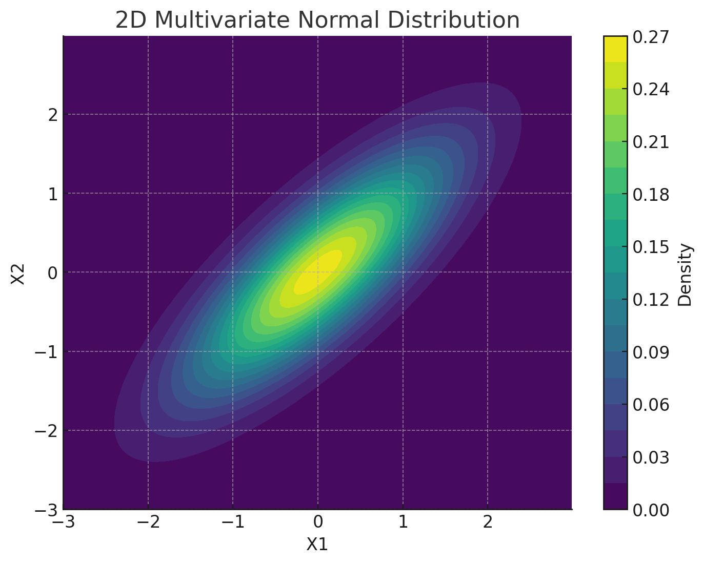
Multi-Variate Gaussian

definition

---

• 다변량 가우시안 분포(Multi-Variate Normal Distribution): 유한 차원의 상관된 가우시안 확률변수 벡터에 대하여 정의되는 가우시안 분포

  \[\begin{aligned} \mathbf{x} \sim \mathcal{N}_{P}\left(\mu, \Sigma\right) \end{aligned}\]

  • \(\mathbf{x}\) : multi-variable vector

    \[\mathbf{x} =\begin{bmatrix} x_{1}&x_{2}&\cdots&x_{p} \end{bmatrix}^{T}\]

  • each elements \(x_{i}\in\mathbf{x}\) are random variables that follow individual Gaussian dist.

    \[x_{i}\sim\mathcal{N}\left(\mu_{i}, \sigma_{i}^{2}\right), \quad x_{i} \cancel{\perp} x_{j}\]

  • \(\mu\): mean vector

    \[\mu =\begin{bmatrix} \mu_{1}&\mu_{2}&\cdots&\mu_{p} \end{bmatrix}^{T}\]

  • \(\Sigma\): covariance matrix

    \[\Sigma =\begin{bmatrix} \sigma_{1}^{2} & \sigma_{1,2} & \cdots & \sigma_{1,p}\\ \sigma_{2,1} & \sigma_{2}^{2} & \cdots & \sigma_{2,p}\\ \vdots & \vdots & \ddots & \vdots\\ \Sigma_{p,1} & \sigma_{p,2} & \cdots & \sigma_{p}^{2} \end{bmatrix}\]

• probability density function:

  \[\begin{aligned} p(\mathbf{x}\mid\mu,\Sigma) &= \frac{1}{(2\pi)^{p/2}\mathrm{det}(\Sigma)^{1/2}} \exp{\left[-\frac{1}{2}\underbrace{(\mathbf{x}-\mu)^{T}\Sigma^{-1}(\mathbf{x}-\mu)}_{\text{Mahalanobis Distance}}\right]} \end{aligned}\]

• moment generating function:

  \[\begin{aligned} M_{X}(\mathbf{t}) &=\mathbb{E}_{p(\mathbf{x})}\left[\exp{t^{T}X}\right]\\ &=\int_{-\infty}^{\infty}{\exp{\mathbf{t}^{T}\mathbf{x}}\cdot p(\mathbf{x})\mathrm{d}\mathbf{x}}\\ &=\frac{1}{(2\pi)^{p/2}\mathrm{det}(\Sigma)^{1/2}}\int_{-\infty}^{\infty}{\exp{\left[\mathbf{t}^{T}\mathbf{x}-\frac{1}{2}\left(\mathbf{x}-\mu\right)^{T}\Sigma^{-1}\left(\mathbf{x}-\mu\right)\right]}\mathrm{d}\mathbf{x}}\\ \\ \mathbf{t}^{T}\mathbf{x}-\frac{1}{2}\left(\mathbf{x}-\mu\right)^{T}\Sigma^{-1}\left(\mathbf{x}-\mu\right) &=-\frac{1}{2}\left(\mathbf{x}-\left[\mu+\Sigma t\right]\right)^{T}\Sigma^{-1}\left(\mathbf{x}-\left[\mu+\Sigma t\right]\right)+\mathbf{t}^{T}\mu+\frac{1}{2}\mathbf{t}^{T}\Sigma\mathbf{t}\\ &=-\frac{1}{2}\left(\mathbf{x}-\mu^{\prime}\right)^{T}\Sigma^{-1}\left(\mathbf{x}-\mu^{\prime}\right)+\mathbf{t}^{T}\mu+\frac{1}{2}\mathbf{t}^{T}\Sigma\mathbf{t}\\ \\ \therefore M_{X}(\mathbf{t}) &=\frac{1}{(2\pi)^{p/2}\mathrm{det}(\Sigma)^{1/2}}\int_{-\infty}^{\infty}{\exp{\left[\mathbf{t}^{T}\mu+\frac{1}{2}\mathbf{t}^{T}\Sigma\mathbf{t}\right]}\cdot\exp{\left[-\frac{1}{2}\left(\mathbf{x}-\mu^{\prime}\right)^{T}\Sigma^{-1}\left(\mathbf{x}-\mu^{\prime}\right)\right]}\mathrm{d}\mathbf{x}}\\ &=\exp{\left[\mathbf{t}^{T}\mu+\frac{1}{2}\mathbf{t}^{T}\Sigma\mathbf{t}\right]}\cdot\underbrace{\frac{1}{(2\pi)^{p/2}\mathrm{det}(\Sigma)^{1/2}}\int_{-\infty}^{\infty}{\exp{\left[-\frac{1}{2}\left(\mathbf{x}-\mu^{\prime}\right)^{T}\Sigma^{-1}\left(\mathbf{x}-\mu^{\prime}\right)\right]}\mathrm{d}\mathbf{x}}}_{=1}\\ &=\exp{\left[\mathbf{t}^{T}\mu+\frac{1}{2}\mathbf{t}^{T}\Sigma\mathbf{t}\right]} \end{aligned}\]
  • $\mathbb{E}\left[X\right]=\nabla_{t}M_{X}(t)\vert_{t=0}=\mu$
  • $\mathbb{E}\left[XX^{T}\right]=\nabla_{t}^{2}M_{X}(t)\vert_{t=0}=\mu^{T}\mu+\Sigma$
  • $\mathrm{Cov}\left[X,X^{\prime}\right]=\mathbb{E}\left[XX^{T}\right]-\mathbb{E}\left[X\right]\mathbb{E}\left[X\right]^{T}=\Sigma$

• canonical form:

  \[\begin{aligned} p(\mathbf{x}) &=\frac{\mathrm{det}(\Lambda)^{1/2}}{(2\pi)^{p/2}}\exp{\left[-\frac{1}{2}(\mathbf{x}-\mu)^{T}\Lambda(\mathbf{x}-\mu)\right]}\\ \\ -\frac{1}{2}(\mathbf{x}-\mu)^{T}\Lambda(\mathbf{x}-\mu) &=-\frac{1}{2}\mathbf{x}^{T}\Lambda\mathbf{x}+\mu^{T}\Lambda\mathbf{x}-\frac{1}{2}\mu^{T}\Lambda\mu\\ \\ \mathbf{x}^{T}\Lambda\mathbf{x} &=\mathrm{tr}\left(\mathbf{x}^{T}\Lambda\mathbf{x}\right)\\ &=\mathrm{tr}\left(\Lambda\mathbf{x}\mathbf{x}^{T}\right)\\ &=\left\langle\Lambda,\mathbf{x}\mathbf{x}^{T}\right\rangle_{F}\\ \\ \therefore -\frac{1}{2}(\mathbf{x}-\mu)^{T}\Lambda(\mathbf{x}-\mu) &=-\frac{1}{2}\left\langle\Lambda,\mathbf{x}\mathbf{x}^{T}\right\rangle_{F}+\mu^{T}\Lambda\mathbf{x}-\frac{1}{2}\mu^{T}\Lambda\mu\\ \\ \therefore p(\mathbf{x}) &=\exp{\left[-\frac{p}{2}\log{2\pi}+\frac{1}{2}\log{\mathrm{det}(\Lambda)}-\frac{1}{2}\left\langle\Lambda,\mathbf{x}\mathbf{x}^{T}\right\rangle_{F}+\mu^{T}\Lambda\mathbf{x}-\frac{1}{2}\mu^{T}\Lambda\mu\right]}\\ &=\frac{1}{(2\pi)^{p/2}}\exp{\left(\begin{bmatrix}-(1/2)\Lambda\\\mu^{T}\Lambda\end{bmatrix}^{T}\begin{bmatrix}\mathbf{x}\mathbf{x}^{T}\\\mathbf{x}\end{bmatrix}-\frac{1}{2}\left[\mu^{T}\Lambda\mu+\log{\mathrm{det}(\Lambda)}\right]\right)} \end{aligned}\]
  • $T(\mathbf{x})=\mathbf{x}\mathbf{x}^{T},\mathbf{x}$
  • $\eta(\theta)=-(1/2)\Lambda,\mu^{T}\Lambda$
  • $A(\eta)=-(1/2)[\mu^{T}\Lambda\mu+\log{\mathrm{det}(\Lambda)}]$
  • $h(\mathbf{x})=1/(2\pi)^{p/2}$

conjugate prior

---

• multi-variate gaussian model:

  \[\mathbf{x}_{i}\mid\Lambda\overset{\mathrm{i.i.d}}{\sim}\mathcal{N}(0,\Lambda^{-1}),\quad i=1,\cdots,n\]

• canonical form:

  \[\begin{aligned} p(\mathbf{x}_{1},\cdots,\mathbf{x}_{n}\mid\Lambda) &=\prod_{i=1}^{n}{p(\mathbf{x}_{i}\mid\Lambda)}\quad(\because \mathbf{x}_{i}\perp \mathbf{x}_{j})\\ &=\prod_{i=1}^{n}{(2\pi)^{-p/2}\mathrm{det}(\Lambda)^{1/2}\exp{\left[-\frac{1}{2}\mathbf{x}_{i}^{T}\Lambda\mathbf{x}_{i}\right]}}\\ &=(2\pi)^{-np/2}\mathrm{det}(\Lambda)^{n/2}\exp{\left[-\frac{1}{2}\sum_{i=1}^{n}{\mathbf{x}_{i}^{T}\Lambda\mathbf{x}_{i}}\right]}\\ \\ \sum_{i=1}^{n}{\mathbf{x}_{i}^{T}\Lambda\mathbf{x}_{i}} &=\sum_{i=1}^{n}{\mathrm{tr}\left(\Lambda\mathbf{x}_{i}\mathbf{x}_{i}^{T}\right)}\\ &=\mathrm{tr}\left(\Lambda\sum_{i=1}^{n}{\mathbf{x}_{i}\mathbf{x}_{i}^{T}}\right)\\ &=\mathrm{tr}(\Lambda S)\quad\mathrm{for}\quad S:=\sum_{i=1}^{n}{\mathbf{x}_{i}\mathbf{x}_{i}^{T}}\\ \\ \mathrm{tr}(\Lambda S) &=\sum_{i=1}^{p}{(\Lambda S)_{i,i}}\\ &=\sum_{i=1}^{p}\sum_{j=1}^{p}{\Lambda_{i,j}S_{j,i}}\\ &=\sum_{i=1}^{p}\sum_{j=1}^{p}{\Lambda_{i,j}S_{i,j}}\quad(\because S=S^{T})\\ &=\langle\Lambda,S\rangle_{F}\\ \\ \therefore p(\mathbf{x}_{1},\cdots,\mathbf{x}_{n}\mid\Lambda) &= (2\pi)^{-np/2}\mathrm{det}(\Lambda)^{n/2}\exp{\left[-\frac{1}{2}\langle\Lambda,S\rangle_{F}\right]}\\ &= (2\pi)^{-np/2}\exp{\left(-\frac{1}{2}\langle\Lambda,S\rangle_{F}-\left[-\frac{n}{2}\log{\mathrm{det}(\Lambda)}\right]\right)} \end{aligned}\]
  • $T(x)=S$
  • $\eta(\theta)=-(1/2)\Lambda$
  • $A(\eta)=-(n/2)\log{\mathrm{det}(\Lambda)}$
  • $h(x)=(2\pi)^{-np/2}$

• prior of $\eta$:

  \[\begin{aligned} p(\eta) &\propto\exp{\left[\left\langle\chi,\eta(\theta)\right\rangle_{F}-\nu\cdot A(\eta)\right]}\quad\mathrm{for}\quad\chi^{T}=\chi\\ &=\exp{\left(\chi\cdot\eta-\nu\cdot\left[-\frac{1}{2}\log{\mathrm{det}(-2\eta)}\right]\right)} \end{aligned}\]

• change of variables $\eta\to\Lambda$:

  \[\begin{aligned} p_{\Lambda}(\Lambda)\mathrm{d}\Lambda &=p_{\eta}(\eta)\mathrm{d}\eta\\ \therefore p_{\Lambda}(\Lambda) &=p_{\eta}(\eta)\left\vert\frac{\mathrm{d}\eta}{\mathrm{d}\Lambda}\right\vert\\ &\propto\exp{\left(\chi\cdot\left[-\frac{1}{2}\Lambda\right]-\nu\cdot\left[-\frac{1}{2}\log{\mathrm{det}(\Lambda)}\right]\right)}\cdot\left\vert-\frac{1}{2}\right\vert^{p(p+1)/2}\\ &\propto\exp{\left[-\frac{1}{2}\mathrm{tr}\left(\chi^{T}\Lambda\right)+\frac{\nu}{2}\log{\mathrm{det}(\Lambda)}\right]}\\ &=\mathrm{det}(\Lambda)^{\nu/2}\exp{\left[-\frac{1}{2}\mathrm{tr}\left(\chi^{T}\Lambda\right)\right]}\\ &=\mathrm{det}(\Lambda)^{\nu/2}\exp{\left[-\frac{1}{2}\mathrm{tr}\left(\chi\Lambda\right)\right]}\quad(\because\chi^{T}=\chi)\\ &\approx \mathcal{W}_{P}\left(\nu+p+1,\chi^{-1}\right) \end{aligned}\]

• Therefore, the precision of the Multi-Variate Gaussian distribution $\Sigma^{-1}$, the reciprocal of the covariance, follows a Wishart distribution. Here, each parameter of the wishart distribution represents (1) degrees of freedom and (2) the precision scale.

  \[\Sigma^{-1}\sim\mathcal{W}_{P}(\nu,V)\]

conditional probability

---

• 마할라노비스 거리(Mahalanobis Distance): 상관관계가 존재하는 다변량 데이터에서, 하나의 데이터 포인트가 특정 분포 혹은 군집에서 얼마나 떨어져 있는지를 측정하는 개념으로서, 단순 좌표 상의 거리뿐만 아니라 데이터 분포(분산-공분산 구조)까지 반영하여 측정된 거리

  \[\begin{aligned} D_{M}(x) &= \sqrt{(x-\mu)^{T}\Sigma^{-1}(x-\mu)} \end{aligned}\]
  • $\sqrt{(x-\mu)^{T}(x-\mu)}$ : 데이터 포인트와 특정 분포 중심점 간 편차로서 유클리드 거리
  • $\Sigma$ : 특정 분포의 공분산 행렬로서 데이터의 분산과 변수 간 상관관계를 포함하며, 이를 반영하여 방향성과 크기에 따라 거리를 조정함

• multi-variate gaussian dist.:

  \[\begin{aligned} \mathbf{Z} =\begin{bmatrix}Z_{1} \\ Z_{2}\end{bmatrix} \sim \mathcal{N}\left(\begin{bmatrix}\mu_{1} \\ \mu_{2}\end{bmatrix}, \begin{bmatrix}\Sigma_{11} & \Sigma_{12}\\ \Sigma_{21} & \Sigma_{22}\end{bmatrix}\right) \end{aligned}\]

• probability density function:

  \[\begin{aligned} p(\mathbf{Z}) &= \frac{1}{(2\pi)^{n/2}\mathrm{det}(\Sigma)^{1/2}} \exp{\left[-\frac{1}{2}\underbrace{(\mathbf{Z}-\mu)^{T}\Sigma^{-1}(\mathbf{Z}-\mu)}_{\text{Mahalanobis Distance}}\right]} \end{aligned}\]

• inv-covariance matrix:

  \[\begin{aligned} \Sigma^{-1} &= \begin{bmatrix} \Sigma_{11}^{-1}+\Sigma_{11}^{-1}\Sigma_{12} \cdot \left(\Sigma_{22}-\Sigma_{21}\Sigma_{11}^{-1}\Sigma_{12}\right)^{-1} \cdot \Sigma_{12}\Sigma_{11}^{-1} & -\Sigma_{11}^{-1}\Sigma_{12}\left(\Sigma_{22}-\Sigma_{21}\Sigma_{11}^{-1}\Sigma_{12}\right)^{-1}\\ -\left(\Sigma_{22}-\Sigma_{21}\Sigma_{11}^{-1}\Sigma_{12}\right)^{-1}\Sigma_{21}\Sigma_{11}^{-1} & \left(\Sigma_{22}-\Sigma_{21}\Sigma_{11}^{-1}\Sigma_{12}\right)^{-1} \end{bmatrix} \end{aligned}\]

• exponent formula expansion:

  \[\begin{aligned} (\mathbf{Z}-\mu)^{T}\Sigma^{-1}(\mathbf{Z}-\mu) &= \underbrace{(Z_{1}-\mu_{1})^{T}\Sigma_{11}^{-1}(Z_{1}-\mu_{1})}_{\text{Mahalanobis Distance of } Z_{1}}\\ &\quad + \underbrace{\left[Z_{2}-\left\{\mu_{2}+\Sigma_{21}\Sigma_{11}^{-1}(Z_{1}-\mu_{1})\right\}\right]^{T}\left(\Sigma_{22}-\Sigma_{21}\Sigma_{11}^{-1}\Sigma_{12}\right)^{-1}\left[Z_{2}-\left\{\mu_{2}+\Sigma_{21}\Sigma_{11}^{-1}(Z_{1}-\mu_{1})\right\}\right]}_{\text{Conditional Mahalanobis Distance of }Z_{2} \mid Z_{1}} \end{aligned}\]

• components of the conditional Mahalanobis distance can be interpreted in terms of expectation and covariance:

  \[\begin{aligned} \mathbb{E}\left[Z_{2} \mid Z_{1}\right] &= \mu_{2} + \Sigma_{21}\Sigma_{11}^{-1}(Z_{1}-\mu_{1})\\ \mathrm{Cov}\left[Z_{2} \mid Z_{1}\right] &= \Sigma_{22}-\Sigma_{21}\Sigma_{11}^{-1}\Sigma_{12} \end{aligned}\]