Neural Network

Neural Network

---

Perceptron

• 퍼셉트론(Perceptron) : 다수의 신호를 입력 받아 하나의 신호를 출력하는 알고리즘

  

  \[\begin{aligned} y = \begin{cases} 0 \quad & \overrightarrow{\mathbf{w}} \cdot \overrightarrow{\mathbf{x}} \le \theta \\ 1 \quad & \overrightarrow{\mathbf{w}} \cdot \overrightarrow{\mathbf{x}} > \theta \\ \end{cases}, \quad x \in \{0,1\} \end{aligned}\]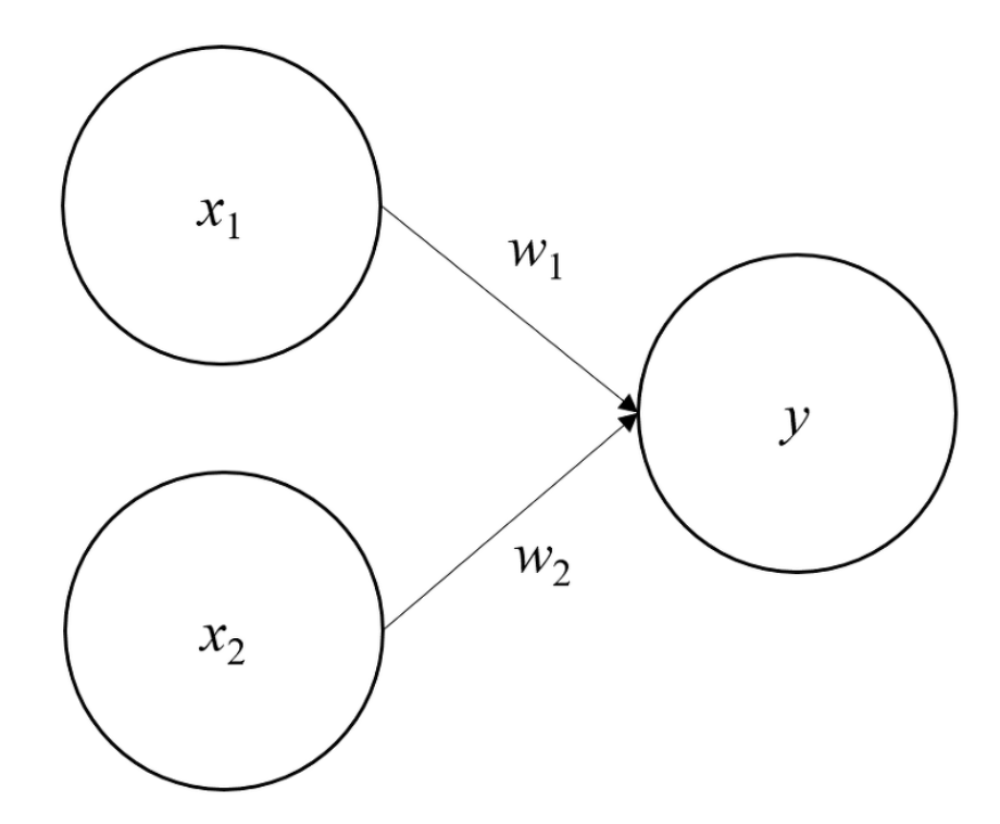

• 논리 회로(Logic Gate) : 하나 이상의 논리 입력을 받아 일정한 논리 연산을 거쳐 논리 출력을 얻는 회로

  

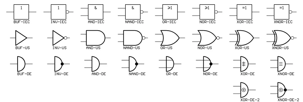
  Gate	Desc
  AND	입력값이 모두 $1$ 이면 $1$ 을 출력함
  OR	입력값이 하나라도 $1$ 이면 $1$ 을 출력함
  NOT	입력값이 $0$ 이면 $1$ 을, $1$ 이면 $0$ 을 출력함
  NAND	입력값이 모두 $1$ 이면 $0$ 을 출력함
  NOR	입력값이 하나라도 $1$ 이면 $0$ 을 출력함
  XOR	입력값이 서로 다르면 $1$ 을, 같으면 $0$ 을 출력함
  XNOR	입력값이 서로 다르면 $0$ 을, 같으면 $1$ 을 출력함

• MLP(Multi-Layer Perceptron)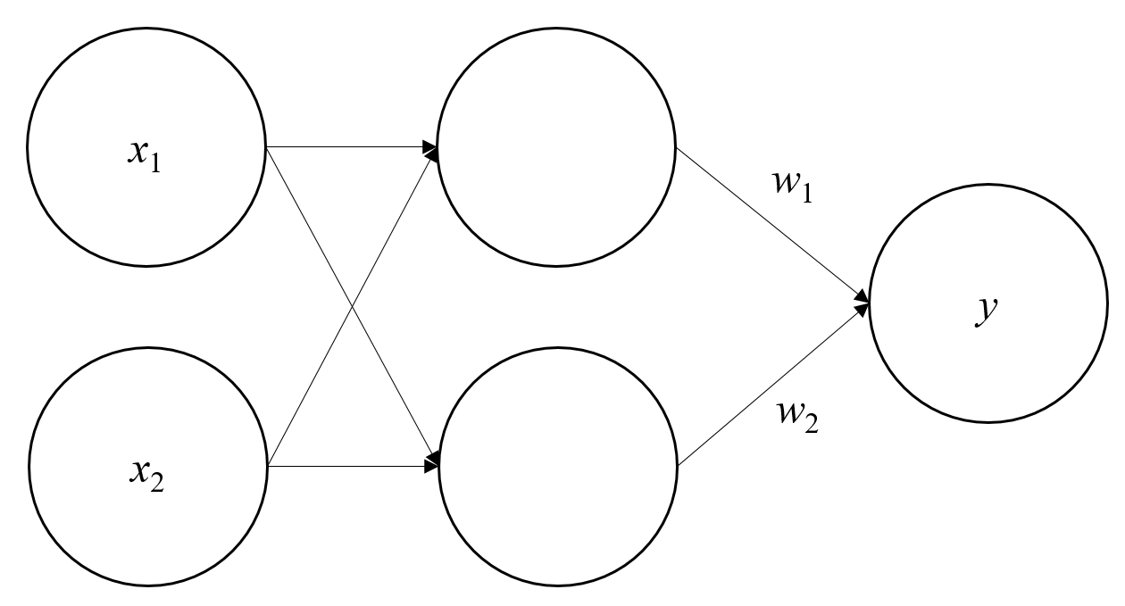

  

  • 단층 퍼셉트론은 선형 분류기로서 게이트를 다양한 가중치 조합을 통해 표현할 수 있으나, 비선형 분류기를 요하는 일부 게이트(XOR, XNOR)에 대해서는 표현이 불가능함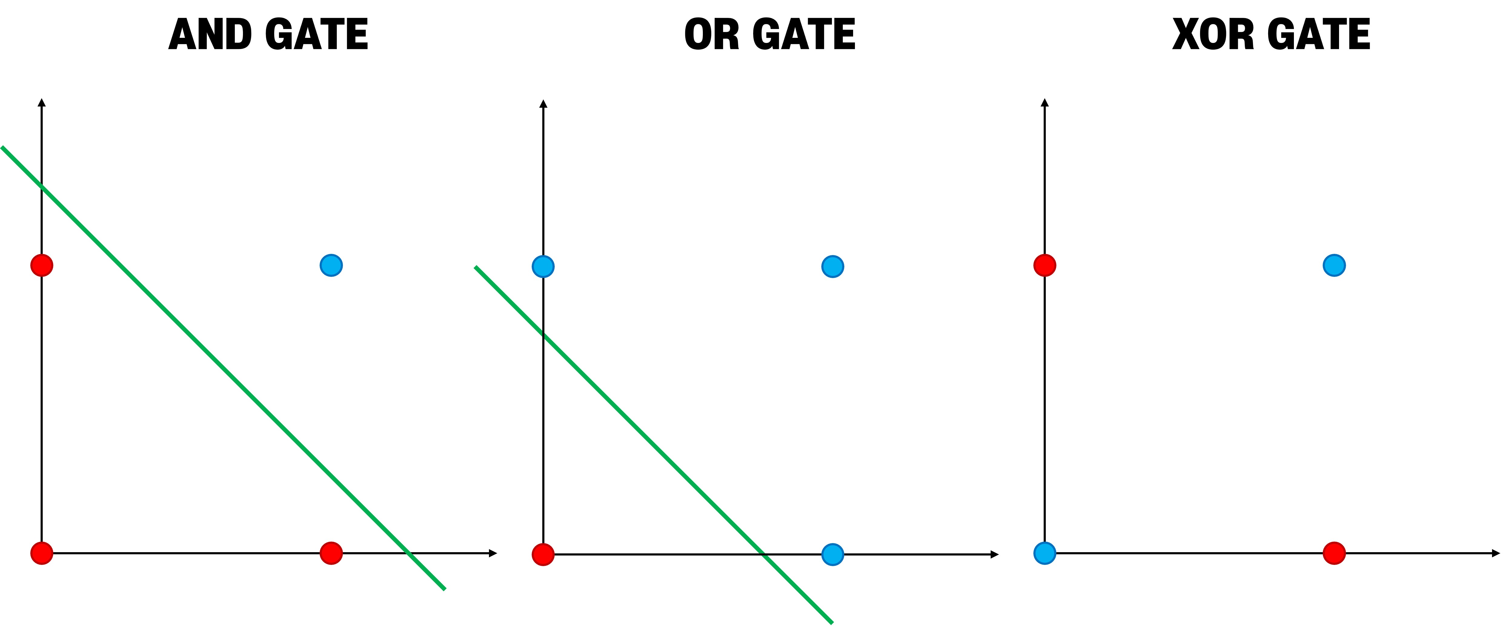

    

  • 이는 NAND, OR, AND 게이트를 표현하는 퍼셉트론들의 조합으로 표현할 수 있음

    

    $X_{1}$	$X_{2}$	$Z_{1}$ NAND	$Z_{2}$ OR	$Y$ AND
    $0$	$0$	$1$	$0$	$0$
    $0$	$1$	$1$	$1$	$1$
    $1$	$0$	$1$	$1$	$1$
    $1$	$1$	$0$	$1$	$0$

Neural Network

• 인공신경망(Artifical Neural Network) : 생물학적 신경망에서 영감을 얻은 통계학적 학습 알고리즘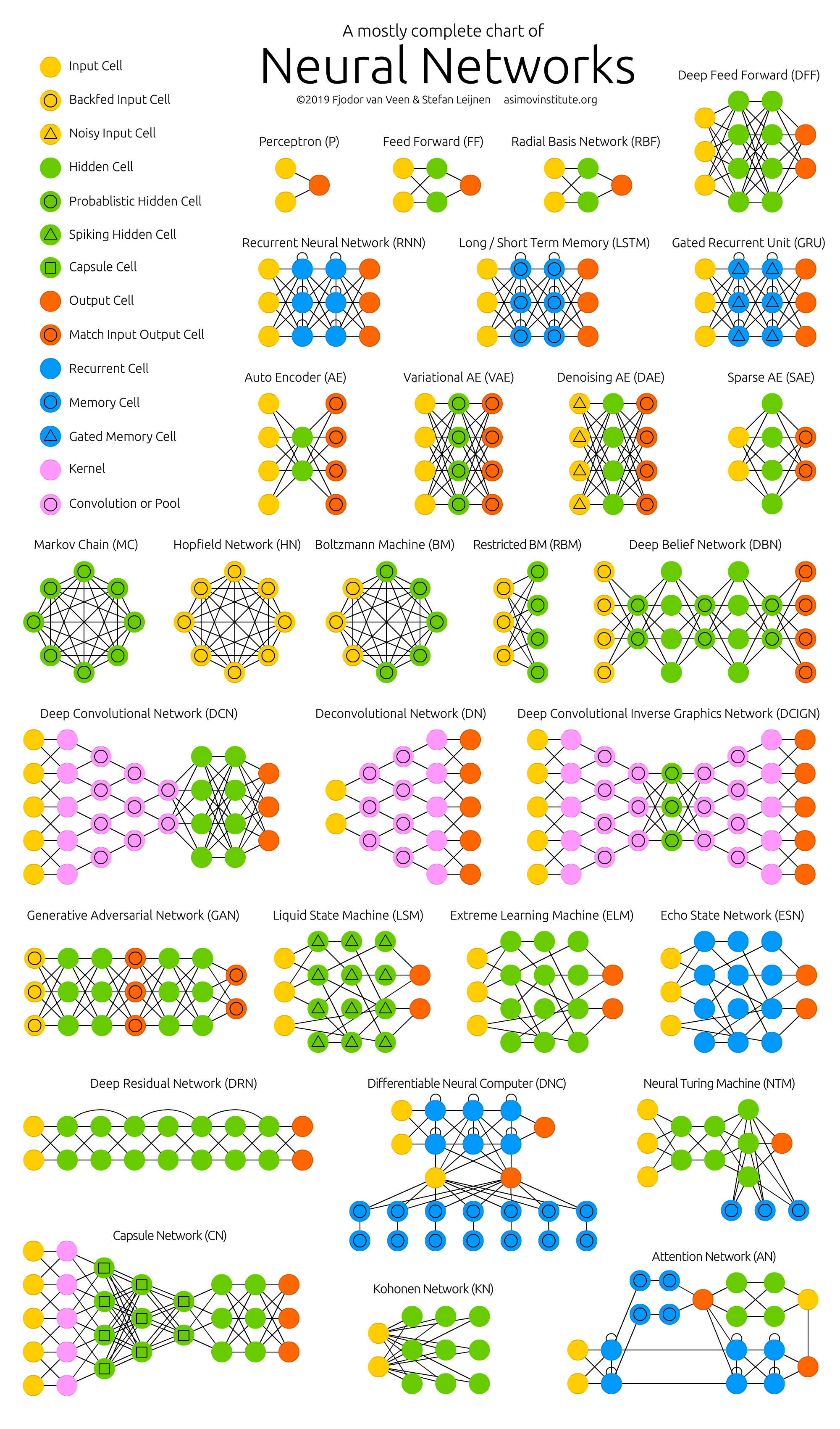

  

• MLP(Multi-Layer Perceptron) is FC(Fully-Connected) FFNN(Feed-Forward Neural Network)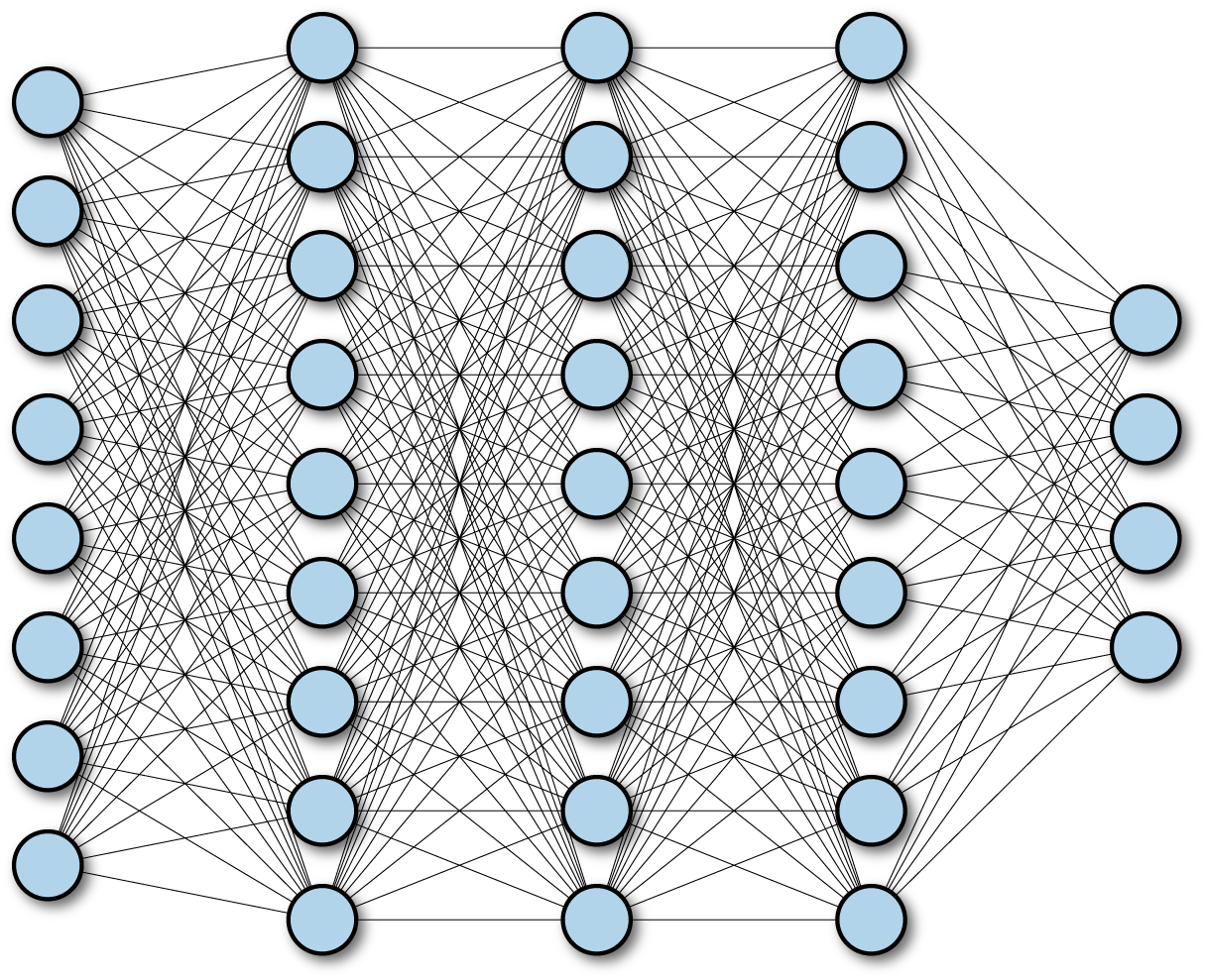

  

  • Layer : 하나 이상의 퍼셉트론으로 구성된 모듈
  • FC(Fully-Connected) : 레이어의 모든 뉴런이 다음 레이어의 모든 뉴런과 연결된 상태
  • FFNN(Feed-Forward Neural Network) : 신호가 하나의 방향으로만 전달되는 인공신경망

• MLP Definition

  

  \[\begin{aligned} \hat{y} &= \text{MLP}(\overrightarrow{\mathbf{x}})\\ &= F^{(N)} \circ \cdots \circ F^{(i)} \circ \cdots \circ F^{(1)}(\overrightarrow{\mathbf{x}}) \end{aligned}\]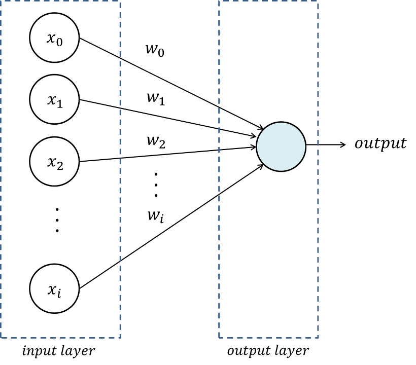
  • $F^{(i)} = h \circ g$ : Single Layer
  • \(\overrightarrow{\mathbf{y}}^{(i)}\) : Activation Value
  • $h(\overrightarrow{\mathbf{z}}^{(i)})$ : Activation Function
  • \(\overrightarrow{\mathbf{z}}^{(i)}\) : Net Input
  • \(g(\overrightarrow{\mathbf{y}}^{(i-1)})=\mathbf{W}^{(i)} \cdot \overrightarrow{\mathbf{y}}^{(i-1)} + \overrightarrow{\mathbf{b}}^{(i)}\) : Summed Input Function or Weighted Sum Function

• 활성화 함수(Activation Function) : 다음 레이어 뉴런으로의 전달 여부를 판단하는 함수($h(\cdot)$)

  

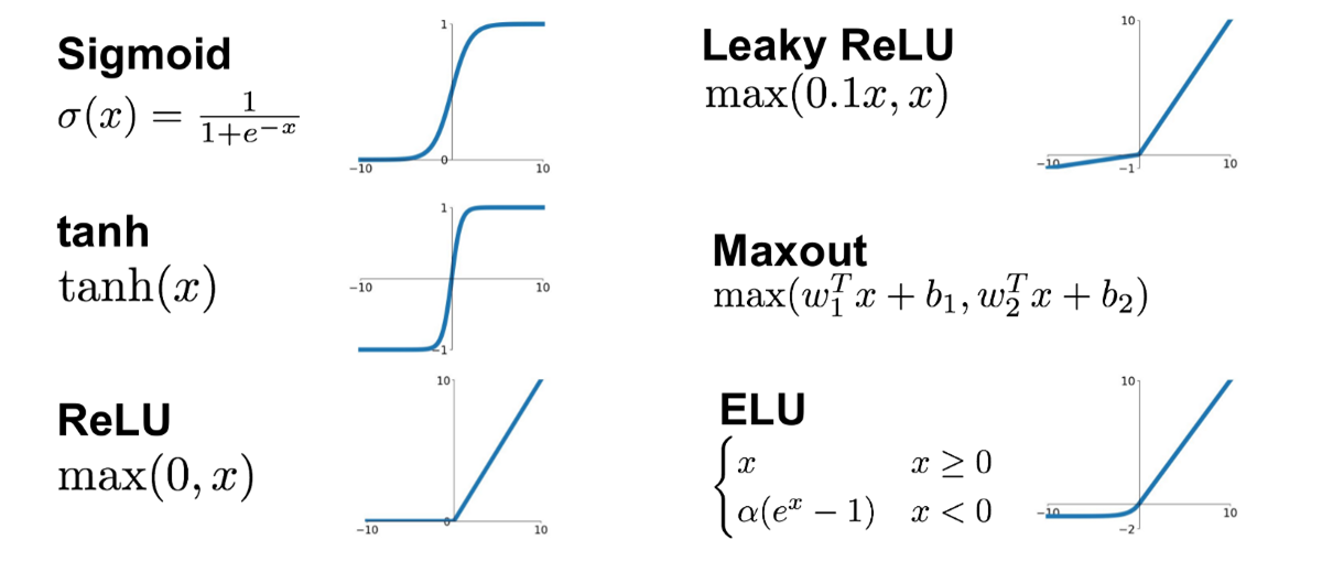
  	Function	Output
  Step	\(\text{step}(x)=\begin{cases} 1, \ \text{if} \ x>0 \\ 0, \ \text{otherwise} \end{cases}\)	\(y \in \{0, 1\}\)
  Sigmoid	\(\text{sigmoid}(x)=\displaystyle\frac{1}{1+e^{-x}}\)	\(y \in [0, 1]\)
  TANH	\(\begin{aligned}\text{tanh}(x)&=\frac{\text{sinh}(x)}{\text{cosh}(x)} \\ &=\frac{e^{x}-e^{-x}}{e^{x}+e^{-x}}\end{aligned}\)	\(y \in [-1, 1]\)
  ReLU	\(\text{ReLU}(x)=\max(0,x)\)	\(y \in [0, \infty]\)
  Softmax	\(\text{softmax}(x)_{i} = \displaystyle\frac{\exp{x_i}}{\sum_{j \ne i}{\exp{x_j}}}\)	\(y \in [0, 1]\)

Backward Propagation

---

Gradient Descent

• 그라디언트(Gradient) : 다변수 함수에 대하여 모든 방향으로의 순간변화율 벡터

  

  \[\begin{aligned} \nabla{f(x_{1},x_{2},\cdots,x_{n})} &= \begin{pmatrix} \displaystyle\frac{\partial f(x^{\forall})}{\partial x_{1}}\\ \displaystyle\frac{\partial f(x^{\forall})}{\partial x_{2}}\\ \vdots\\ \displaystyle\frac{\partial f(x^{\forall})}{\partial x_{n}}\\ \end{pmatrix} \end{aligned}\]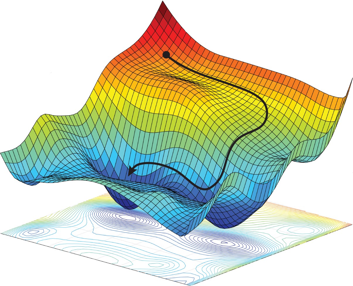

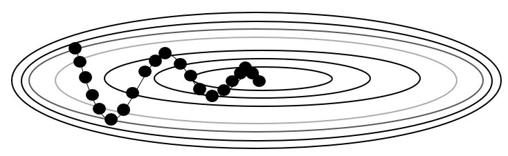
• 경사하강법(Gradient Descent) : 손실 함수의 도함수(그라디언트)를 최소화하는 가중치를 추정하는 방법

  

  \[\begin{aligned} \Theta \gets \Theta - \eta \cdot \nabla_{\Theta}\mathcal{L} \end{aligned}\]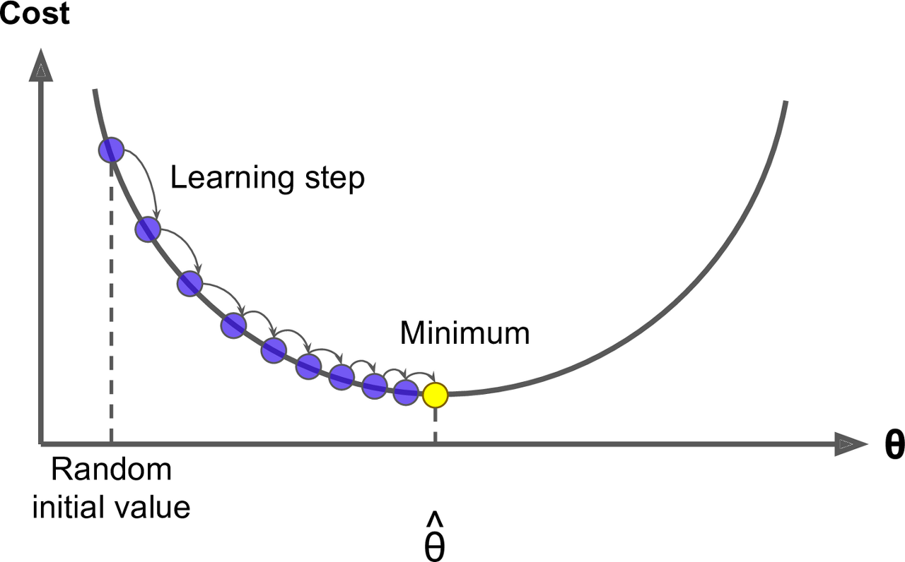
  • $\Theta$ : Learning Parameter
  • $\eta$ : Learning Rate or Learning Step
  • $\nabla_{\Theta}\mathcal{L}$ : Gradient of the Loss Function is Learning Direction

Backward Propagation

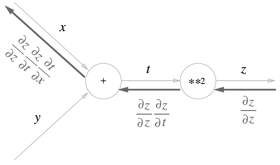
• 역전파(Backward Propagation) : 경사하강법을 활용하여 오차를 출력층에서 입력층 방향으로 전파하며 가중치를 조정하는 학습 방법

  

• Learning Direction

  • 손실 $\mathcal{L}$ 를 $1$ 번째 계층의 $1$ 번째 가중치 $w^{(1)}_{1}$ 에 대하여 미분하면 다음과 같음

    \[\begin{aligned} \frac{\partial}{\partial w^{(1)}_{1}}\mathcal{L}(y,\hat{y}) &= \frac{\partial \mathcal{L}}{\partial\cancel{\overrightarrow{\mathbf{y}}^{(N)}}} \times \frac{\partial\cancel{\overrightarrow{\mathbf{y}}^{(N)}}}{\partial\cancel{\overrightarrow{\mathbf{z}}^{(N)}}} \times \frac{\partial\cancel{\overrightarrow{\mathbf{z}}^{(N)}}}{\partial\cancel{\overrightarrow{\mathbf{y}}^{(N-1)}}} \times \cdots \times \frac{\partial\cancel{\overrightarrow{\mathbf{y}}^{(1)}}}{\partial\cancel{\overrightarrow{\mathbf{z}}^{(1)}}} \times \frac{\partial\cancel{\overrightarrow{\mathbf{z}}^{(1)}}}{\partial w^{(1)}_{1}} \end{aligned}\]

  • 위 각 항목을 일반화하면 다음과 같음

    \[\begin{aligned} \frac{\partial \mathcal{L}}{\partial \overrightarrow{\mathbf{y}}^{(N)}} =1, \quad \frac{\partial \overrightarrow{\mathbf{y}}^{(i)}}{\partial \overrightarrow{\mathbf{z}}^{(i)}} =h^{\prime}(\overrightarrow{\mathbf{z}}^{(i)}), \quad \frac{\partial \overrightarrow{\mathbf{z}}^{(i)}}{\partial \overrightarrow{\mathbf{y}}^{(i-1)}} =\mathbf{W}^{(i)}, \quad \frac{\partial \overrightarrow{\mathbf{z}}^{(k)}}{\partial \mathbf{W}^{(k)}} =\overrightarrow{\mathbf{y}}^{(k-1)} \end{aligned}\]

  • 따라서 파라미터 갱신 방향은 다음과 같이 일반화할 수 있음

    \[\begin{aligned} \frac{\partial \mathcal{L}}{\partial \mathbf{W}^{(k)}} &= \overrightarrow{\mathbf{y}}^{(k-1)} \times \prod_{i=k+1}^{N}{\mathbf{W}^{(i)}} \times \prod_{i=k}^{N}{h^{\prime}(\overrightarrow{\mathbf{z}}^{(i)})} \end{aligned}\]

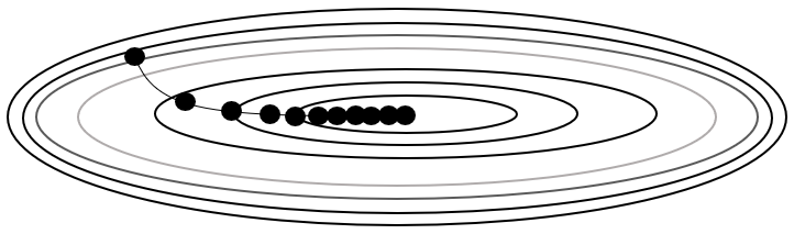
Optimizer

• Update Learning Rate-based Approach

  

  • Adagrad : 이전까지 누적 갱신 규모를 반영하여 학습률을 결정함

    \[\begin{aligned} \Theta_{t} &= \Theta_{t-1} - \frac{\eta}{\sqrt{\phi_{t}}} \times \frac{\partial \mathcal{L}_{t-1}}{\partial \Theta_{t-1}}\\ \phi_{t} &= \phi_{t-1} + \frac{\partial \mathcal{L}_{t}}{\partial \Theta_{t}} \odot \frac{\partial \mathcal{L}_{t}}{\partial \Theta_{t}} \end{aligned}\]

  • RMSProp : 이전까지 누적 갱신 규모를 지수가중이동평균하여 반영하여 학습률을 결정함

    \[\begin{aligned} \Theta_{t} &= \Theta_{t-1} - \frac{\eta}{\sqrt{\phi_{t}}} \times \frac{\partial \mathcal{L}_{t-1}}{\partial \Theta_{t-1}}\\ \phi_{t} &= \rho \cdot \phi_{t-1} + (1-\rho) \cdot \frac{\partial \mathcal{L}_{t}}{\partial \Theta_{t}} \odot \frac{\partial \mathcal{L}_{t}}{\partial \Theta_{t}} \end{aligned}\]

• Update Learning Direction-based Approach

  

  • Momentum : 직전 시점 갱신 방향을 관성 계수($\gamma$)만큼 반영하여 갱신 방향을 결정함

    \[\begin{aligned} \Theta_{t} &= \Theta_{t-1} - \phi_{t}\\ \phi_{t} &= \eta \cdot \frac{\partial \mathcal{L}_{t-1}}{\partial \Theta_{t-1}} + \gamma \cdot \phi_{t-1} \end{aligned}\]

---

Reference

• https://codetorial.net/tensorflow/basics_of_optimizer.html
• https://namu.wiki/jump/JsjHPjk9qYK%2Fl54QLaGyq5jupzXBHwWbSS0dMWuO%2B3lzPTdSDH1TiTY1jg9ysGRCY1f5J8NIWqRsnWauQXGsLQ%3D%3D
• https://gentlesark.tistory.com/44
• https://www.asimovinstitute.org/neural-network-zoo/
• https://www.oreilly.com/library/view/tensorflow-for-deep/9781491980446/ch04.html
• https://towardsdatascience.com/an-intuitive-explanation-of-gradient-descent-83adf68c9c33