Support Vector Machine
Based on the lecture “Intro. to Machine Learning (2023-2)” by Prof. Je Hyuk Lee, Dept. of Data Science, The Grad. School, Kookmin Univ.

Support Vector Machine
-
서포트 벡터 머신(
SupportVectorMachine): 마진(Margin)을 최대로 가져가는 초평면(Hyper Plane)을 규칙으로 하여 관측치를 분류하는 알고리즘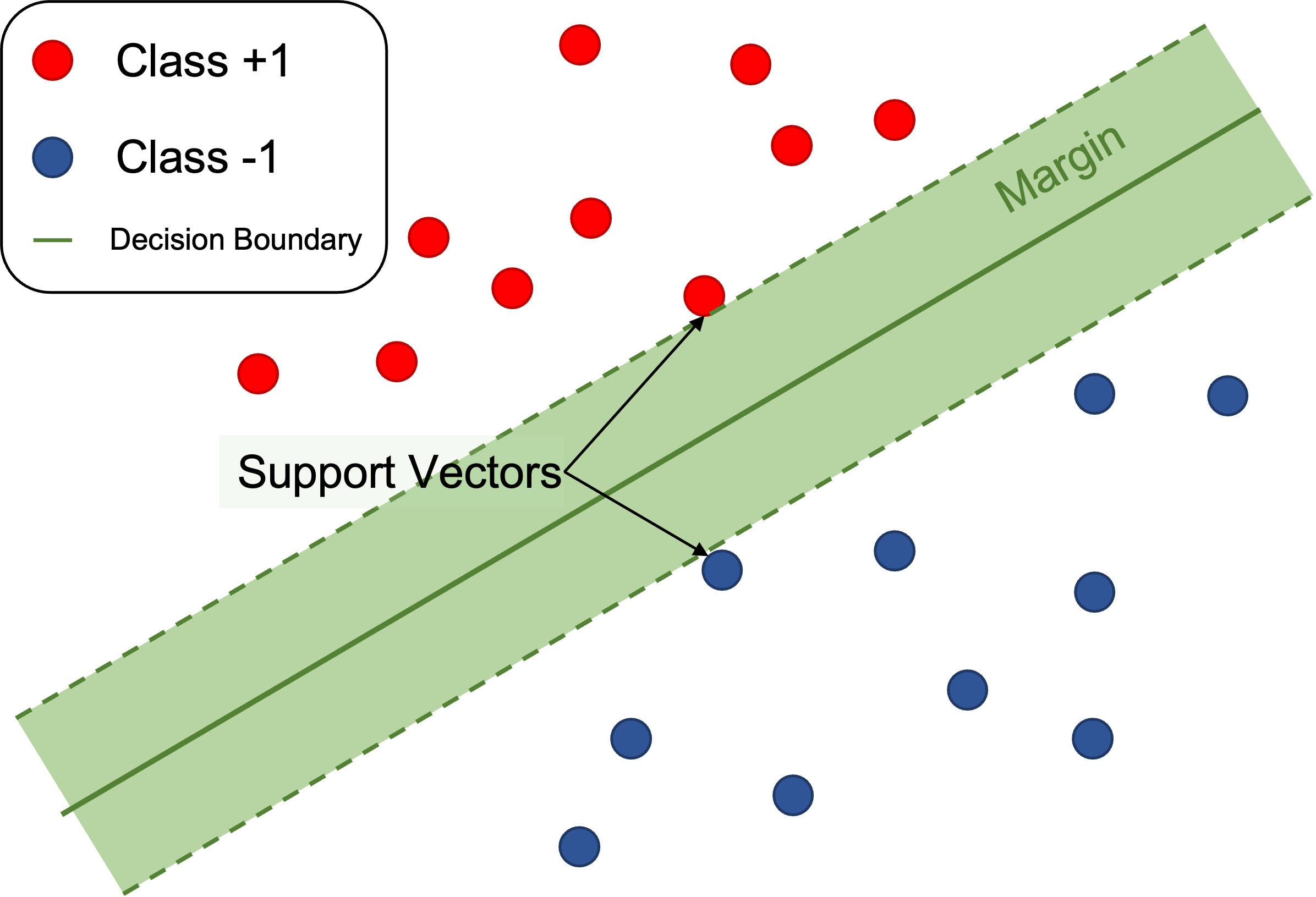
- 초평면(Hyper Plane) : 범주를 구분하는 경계
- 서포트 벡터(Support Vector) : 인접한 범주에 가장 가까이 위치한 벡터
- 마진(Margin) : 인접한 두 범주의 서포트 벡터를 지나는 평행한 두 직선 사이의 유클리드 거리
Decision Function
-
Class of New Obs \(\mathbf{q}\):
\[\begin{aligned} y_{q} &= \begin{cases} +1, \quad &\text{if} \quad f(\mathbf{q}) > 0 \\ -1, \quad &\text{if} \quad f(\mathbf{q}) < 0 \\ \end{cases} \end{aligned}\] -
Decision Function is the Projection Distance between the Hyperplane and the Vector:
\[\begin{aligned} f(\mathbf{q}) &= \mathbf{w}^{*} \cdot \mathbf{q} + b^{*}\\ &= \left(\sum_{i \in SV}{\lambda_{i}y_{i}\mathbf{x}_{i}}\right) \cdot \mathbf{q} + \frac{1}{ \vert SV \vert }\sum_{i \in SV}\sum_{j \in SV}{\left[y_{i} - \lambda_{j}y_{j}\mathbf{x}_{j}\mathbf{x}_{i}\right]} \end{aligned}\]
Concept
-
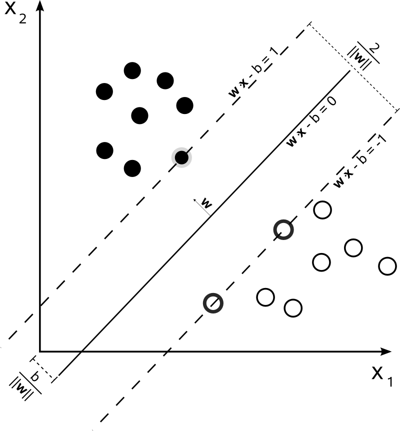
Hyper-Plane
\[\begin{aligned} \mathbf{w}^{T}\mathbf{x}+b &=0 \end{aligned}\]- \(\mathbf{x}\) : 초평면 위에 위치한 벡터
- \(\mathbf{w}\) : 초평면의 법선 벡터
- \(b\) : 편향으로서 세로축 절편
-
Class
\[\begin{aligned} y_{i} = \begin{cases} +1,\quad &\text{if} \quad \mathbf{x}_{i} \in \mathbf{X}^{+}\\ -1,\quad &\text{if} \quad \mathbf{x}_{i} \in \mathbf{X}^{-} \end{cases} \end{aligned}\] -
Support Vector
-
Left Support Vector \(\mathbf{x}^{+}\):
\[\begin{aligned} \mathbf{w}^{T}\mathbf{x}^{+}+b &=+1 \end{aligned}\] -
Right Support Vector \(\mathbf{x}^{-}\):
\[\begin{aligned} \mathbf{w}^{T}\mathbf{x}^{-}+b &=-1 \end{aligned}\]
-
Margin
-
우측 서포트 벡터 \(\mathbf{x}^{-}\) 를 방향 \(\mathbf{w}\) 으로 크기 \(\text{margin}\) 만큼 이동하면 좌측 서포트 벡터 \(\mathbf{x}^{+}\) 에 안착한다고 하자
\[\begin{aligned} \mathbf{x}^{+} &= \mathbf{x}^{-} + \text{margin} \cdot \mathbf{w} \end{aligned}\] -
\(\mathbf{w}^{T}\mathbf{x}^{+}+b=1\) 을 다음과 같이 재정의할 수 있음
\[\begin{aligned} \mathbf{w}^{T}\mathbf{x}^{+}+b &=1\\ \mathbf{w}^{T}\left(\mathbf{x}^{-} + \text{margin} \cdot \mathbf{w}\right)+b &=1\\ \mathbf{w}^{T}\mathbf{x}^{-} + \text{margin} \cdot \mathbf{w}^{T}\mathbf{w} + b &=1\\ \left(\mathbf{w}^{T}\mathbf{x}^{-} + b\right) + \text{margin} \cdot \mathbf{w}^{T}\mathbf{w} &=1\\ -1 + \text{margin} \cdot \Vert \mathbf{w} \Vert ^2 &= 1 \end{aligned}\] -
따라서 마진을 다음과 같이 도출할 수 있음
\[\begin{aligned} \text{margin} &= \frac{2}{ \Vert \mathbf{w} \Vert ^2} \end{aligned}\]
Maximum Margin
-
Definition of Optimization Problem
-
Objective Function:
\[\begin{aligned} \max{\frac{2}{ \Vert \mathbf{w} \Vert ^2}} \Rightarrow \min{\frac{1}{2} \Vert \mathbf{w} \Vert ^2} \end{aligned}\] -
Constraint:
\[\begin{aligned} y_{i}\left(\mathbf{w}^{T}\mathbf{x}_{i}+b\right) \ge 1 \end{aligned}\]
-
-
Lagrangian Function
-
Lagrangian Function:
\[\begin{aligned} \mathcal{L}(\mathbf{w},b,\lambda) &=\frac{1}{2} \Vert \mathbf{w} \Vert ^2 - \sum_{i=1}^{n}{\lambda_{i}\cdot\left[y_{i}\left(\mathbf{w}^{T}\mathbf{x}_{i}+b\right)-1\right]} \end{aligned}\]- $\lambda_{i}\ge 0$ : 라그랑주 승수
-
Complementary Slackness, KKT Conditions:
\[\begin{aligned} \lambda_{i}\cdot\left[y_{i}\left(\mathbf{w}^{T}\mathbf{x}_{i}+b\right)-1\right] &=0 \end{aligned}\]- Support Vector : \(y_{i \in SV}\left(\mathbf{w}^{T}\mathbf{x}_{i \in SV}+b\right)-1=0 \quad \because \mathbf{w}^{T}\mathbf{x}_{i \in SV}+b = 1\)
- Others : \(\lambda_{i \notin SV}=0 \quad \because \mathbf{w}^{T}\mathbf{x}_{i \notin SV}+b > 1\)
-
-
Maximum Margin
\[\begin{aligned} \hat{\Theta} &= \text{arg} \max{\mathcal{L}\left(\mathbf{w},b,\lambda\right)} \end{aligned}\]-
The Normal Vector \(\mathbf{w}^{*}\) that maximizes the margin is:
\[\mathbf{w}^{*} = \sum_{i \in SV}{\lambda_{i}y_{i}\mathbf{x}_{i}}\] -
The Bias \(b^{*}\) that maximizes the margin is:
\[\begin{aligned} b^{*} &= y_{i \in SV} - \mathbf{w}^{T}\mathbf{x}_{i \in SV}\\ &= \frac{1}{ \vert SV \vert }\sum_{i \in SV}{\left[y_{i} - \mathbf{w}^{T}\mathbf{x}_{i}\right]}\\ &= \frac{1}{ \vert SV \vert }\sum_{i \in SV}{\left[y_{i} - \left(\sum_{j \in SV}{\lambda_{j}y_{j}\mathbf{x}_{j}}\right)\mathbf{x}_{i}\right]}\quad \because \mathbf{w}^{*}=\sum_{i}{\lambda_{i}y_{i}\mathbf{x}_{i}}\\ &= \frac{1}{ \vert SV \vert }\sum_{i \in SV}\sum_{j \in SV}{\left[y_{i} - \lambda_{j}y_{j}\mathbf{x}_{j}\mathbf{x}_{i}\right]} \end{aligned}\] -
The Support Vector \(\mathbf{x}_{SV} \in SV\) that maximizes the margin is:
\[\begin{aligned} SV &= \left\{\mathbf{x}_{SV} \mid \mathbf{w}^{*} \cdot \mathbf{x}_{SV} + b^{*} = \vert 1 \vert \right\}\\ &= \left\{\mathbf{x}_{SV} \mid \left(\sum_{i=1}^{n}{\lambda_{i}^{*}y_{i}\mathbf{x}_{i}}\right) \cdot \mathbf{x}_{SV} + \frac{1}{ \vert SV \vert }\sum_{i \in SV}\sum_{j \in SV}{\left[y_{i} - \lambda_{j}y_{j}\mathbf{x}_{j}\mathbf{x}_{i}\right]}= \vert 1 \vert \right\} \end{aligned}\]
-
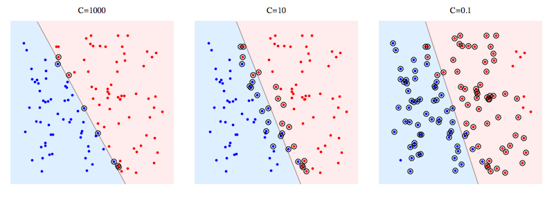
Soft Margin
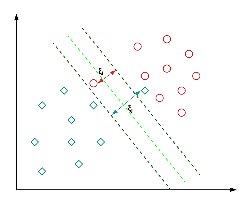
- Soft Margin : 마진 위반 $\xi$ 를 허용하여 일부 이상 관측치를 배제했을 때 마진을 최대화하는 초평면을 탐색함
- 마진 위반(Margin Violation; $\xi$) : 초평면 근방에서 발생 가능한 소수의 이상 관측치에 대한 오류로서, 해당 관측치로부터 서포트 벡터를 지나고 초평면과 평행한 직선까지의 유클리드 거리
-
Definition of Optimization Problem
\[\begin{aligned} \min{\left[\frac{1}{2}{ \Vert \mathbf{w} \Vert ^2}+C\sum_{i=1}^{n}{\xi_i}\right]} \quad \text{s.t.} \quad &y_{i}\left(\mathbf{w}^{T}\mathbf{x}_{i}+b\right) \ge 1-\xi_i,\\ &\xi_i \ge 0 \end{aligned}\]- $\xi_{i}$ : 관측치 벡터 $\mathbf{x}_{i}$ 에 대한 마진 위반
-
$C$ : 마진 위반에 대한 규제 강도
-
Lagrangian Function
\[\begin{aligned} \mathcal{L}(\mathbf{w},b,\lambda,\xi,\mu) &= \left[\frac{1}{2} \Vert \mathbf{w} \Vert ^2 - \sum_{i=1}^{n}{\lambda_{i}\left[y_{i}\left(\mathbf{w}^{T}+b\right)-\left(1-\xi_{i}\right)\right]}\right] + \left[C\sum_{i=1}^{n}{\xi_{i}}-\sum_{i=1}^{b}{\mu_{i}\xi_{i}}\right] \end{aligned}\]- $\lambda \ge 0$ : 제약 조건 \(y_{i}\left(\mathbf{w}^{T}\mathbf{x}+b\right) \ge 1-\xi_{i}\) 에 대한 라그랑주 승수
- $\mu \ge 0$ : 제약 조건 $\xi_{i} \ge 0$ 에 대한 라그랑주 승수
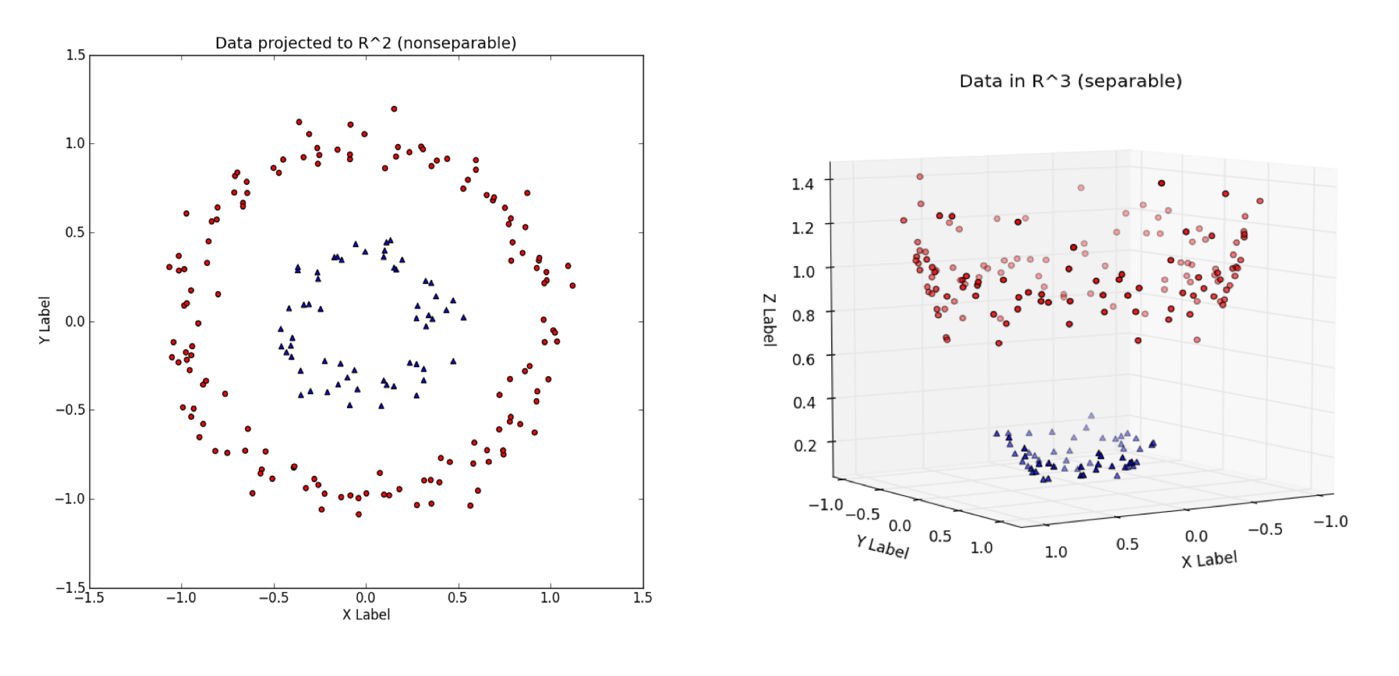
Kernel Trick
-
커널 트릭(Kernel Trick) : 선형으로는 구분하기 어려운 저차원 공간상의 데이터 셋을, 적절한 결정 경계를 찾을 수 있는 고차원 공간으로 매핑하는 기법
-
커널 함수(Kernel Function)
Name Function Linear \(\mathcal{K}\left(X,X^{\prime}\right) = X \cdot X^{\prime}\) Polynomial \(\mathcal{K}\left(X,X^{\prime}\right) = \left(X \cdot X^{\prime} + \beta\right)^{d}\) RBF \(\mathcal{K}\left(X,X^{\prime}\right) = \exp{\left[-\displaystyle\frac{\Vert X-X^{\prime} \Vert^{2}}{2\ell^{2}}\right]}\) Sigmoid \(\mathcal{K}\left(X,X^{\prime}\right) = \text{tanh}\left(\alpha \cdot X \cdot X^{\prime} + \beta\right)\) Laplacian \(\mathcal{K}\left(X,X^{\prime}\right) = \exp{\left[-\gamma \Vert X-X^{\prime} \Vert_{1}\right]}\) Exponential \(\mathcal{K}\left(X,X^{\prime}\right) = \exp{\left[-\gamma \Vert X-X^{\prime} \Vert_{2}\right]}\) Matern \(\mathcal{K}\left(X,X^{\prime}\right) = \displaystyle\frac{2^{1-\nu}}{\Gamma\left(\nu\right)} \cdot \left(\displaystyle\frac{\sqrt{2\nu} \Vert X-X^{\prime} \Vert}{\ell}\right)^{\nu} \cdot K_{\nu}\left(\displaystyle\frac{\sqrt{2\nu} \Vert X-X^{\prime} \Vert}{\ell}\right)\) Periodic \(\mathcal{K}\left(X,X^{\prime}\right) = \exp\left[-2 \sin^2\left( \displaystyle\frac{\pi \vert X-X^{\prime} \vert}{p} \right) \Bigg/ \ell^2 \right]\) Rational Quadratic \(\mathcal{K}\left(X,X^{\prime}\right) = \left( 1 + \displaystyle\frac{\vert X-X^{\prime} \vert^2}{2 \alpha \ell^2} \right)^{-\alpha}\) -
Mercer’s Theorem
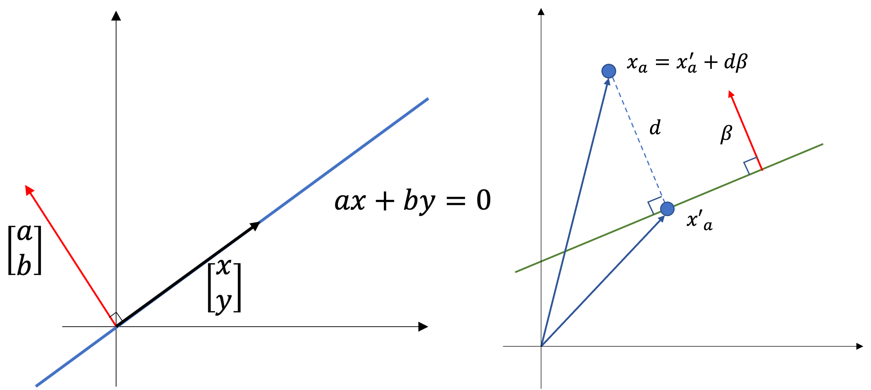
저차원 공간 $L$ 에서 고차원 공간 $H$ 로 관측치들을 매핑하는 커널함수 $K$ 는 $L$ 에서 표현된 관측치들 간 유클리드 거리와 $H$ 에서 표현된 관측치들 간 유클리드 거리를 보존함
-
임의의 관측치 $X_a, X_b$ 에 대하여, $2$ 차원 공간에서 해당 관측치를 나타내는 벡터 $\mathbf{a}, \mathbf{b}$ 를 다음과 같이 정의하자
\[\begin{aligned} \mathbf{a} = \begin{pmatrix}a_1\\a_2\end{pmatrix},\quad \mathbf{b} = \begin{pmatrix}b_1\\b_2\end{pmatrix} \end{aligned}\] -
$\mathbf{a}, \mathbf{b}$ 을 $3$ 차원상의 벡터 $\Phi\left(\mathbf{a}\right),\Phi\left(\mathbf{b}\right)$ 로 매핑하는 커널함수 $K\left(\mathbf{a}, \mathbf{b}\right)$ 는 다음의 조건을 만족함
\[\begin{aligned} K\left(\mathbf{a}, \mathbf{b}\right) &= \left(\mathbf{a}^{T} \mathbf{b}\right)^{2} \\ &= a_{1}^{2} b_{1}^{2} + 2\left(a_{1} b_{1} a_{2} b_{2}\right) + a_{2}^{2}b_{2}^{2} \\ &= \begin{pmatrix}a_{1}^{2}\\ \sqrt{2} a_{1} a_{2}\\ a_{2}^{2}\end{pmatrix} \cdot \begin{pmatrix}b_{1}^{2}\\ \sqrt{2}b_{1} b_{2}\\ b_{2}^{2}\end{pmatrix} \\ &= \Phi\left(\mathbf{a}\right) \cdot \Phi\left(\mathbf{b}\right) \end{aligned}\]
-
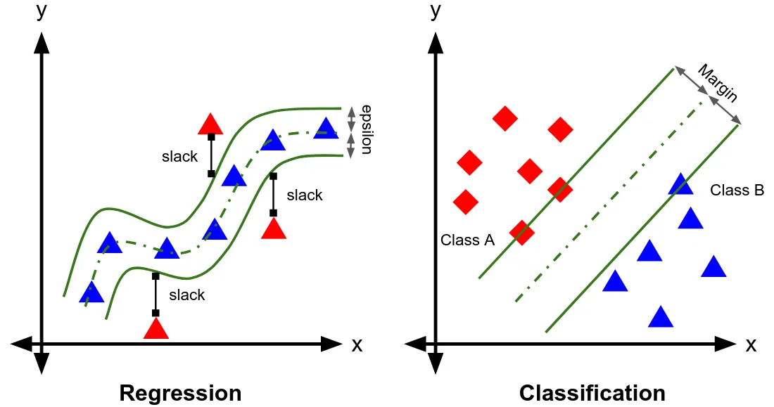
SVR
-
Optimization
\[\begin{aligned} \hat{\Theta} =\text{arg} \min{\left[\frac{1}{2} \Vert \mathbf{w} \Vert^{2} + C\sum_{i=1}^{n}{\left(\xi_{i}+\eta_{i}\right)}\right]} \end{aligned}\] -
Constraint
-
판별 분석 : 마진 범위 이내에 관측치 벡터가 존재하지 않음
\[\begin{aligned} \text{s.t.}\quad &y_{i}\left(\mathbf{w}^{T}\mathbf{x}_{i}+b\right) \ge 1 + \xi_{i}\\ &\xi_{i} \ge 0 \end{aligned}\] -
회귀 분석 : 마진 범위 이내에 모든 관측치 벡터가 존재함
\[\begin{aligned} \text{s.t.} \quad & \varepsilon + \xi_{i} + f\left(\mathbf{x}\right) - y_{i} \ge 0,\\ & \varepsilon + \eta_{i} - f\left(\mathbf{x}\right) + y_{i} \ge 0,\\ & \xi_{i}, \eta_{i} \ge 0 \end{aligned}\]
-
Sourse
- https://velog.io/@shlee0125
- https://medium.com/@niousha.rf/support-vector-regressor-theory-and-coding-exercise-in-python-ca6a7dfda927