BNNs (1) Bayes by Backprop

Bayes by Backprop

---

• 불확실성(Uncertainty): 어떠한 사건에 대하여 확신할 수 없는 상태

  • 우발적 불확실성(Aleatoric Uncertainty): 관측치에 내재된 잡음 혹은 무작위성으로 인해 발생하는 불확실성

  • 인식적 불확실성(Epistemic Uncertainty): 정보 불완전성으로 인하여 발생하는 불확실성
    • 정보 불완전성(Data Uncertainty): 관측 데이터가 불완전하거나(Incomplete), 불충분하거나(Insufficient), 왜곡된(Distorted) 상황
    • 파라미터 불확실성(Parameter Uncertainty): 주어진 모형 안에서 최적 파라미터를 유일하게 식별할 수 없는 문제
    • 구조적 불확실성(Structural Uncertainty): 데이터 생성 메커니즘을 기술하는 함수 구조를 확신할 수 없어 특정 모형을 가정할 수 없는 문제
    • 표현의 불확실성(Latent Representation Uncertainty): 잠재공간의 비식별성으로 인해 치역(관측값)만으로 정의역(잠재요인)을 유일하게 결정하여 표현할 수 없는 문제
  • 존재론적 불확실성(Ontic Uncertainty): 모형이 모사하고자 하는 실제 메커니즘이 본질적으로 불확실하여 정보가 증가하더라도 제거될 수 없는 불확실성

• 문제 의식

  • 모형의 불확실성(Model Uncertainty):

    인공신경망 알고리즘은 파라미터 수가 매우 많아 과적합 문제(Overfitting) 에서 자유롭지 못함. 여기서 과적합이란, 모형의 복잡도가 데이터 셋이 제공하는 정보량보다 심화되어 발생하는 현상임. 이는 정보가 부족한 상황에서 단일 가설을 확신하여 예측하는 과신의 문제(Overconfidence) 에서 비롯함.

  • 사후 분포 계산의 비가용성(intractable):

    과신의 문제를 직접 다루는 베이즈 추론을 신경망에 적용하기에는 사후 분포의 계산이 비가용적임. 다시 말해, 계산 복잡도가 너무 크거나, 해석적으로(analytic) 닫힌형 표현을 얻을 수 없음. 사후 분포 근사 기법인 MCMC, VI 등은 샘플링 과정이 미분 가능하지 않기 때문에 역전파 학습 적용이 불가능함.

• BBB(Bayes by Backprop): 인공신경망의 가중치에 불확실성을 반영하여 데이터에 대한 설명력을 확보하는 동시에(Likelihood) 사전 정보(Prior)를 활용하여 모형의 복잡도를 제어함으로써(Kullback–Leibler divergence) 일반화 성능을 향상시키는 학습 방법론

  • Variational Inference
  • Factorized Gaussian
  • Scale Mixture Gaussian
  • Reparameterization Trick

How to Modeling

---

• Factorized Gaussian is used as the approx. This allows the multivariate Gaussian distribution to be decomposed into the product of independent terms, thereby improving computational efficiency.

  \[\begin{aligned} Q(\mathbf{w}) &=\mathcal{N}(\mu,\sigma^{2}\mathbf{I})\\ &=\prod_{d=1}^{D}{\mathcal{N}(w_{d};\mu_{d},\rho)} \quad \mathrm{s.t.}\quad w_{i} \perp w_{j}\\ \sigma_{d} &=\log{\left[1+\exp{\rho_{d}}\right]} \end{aligned}\]

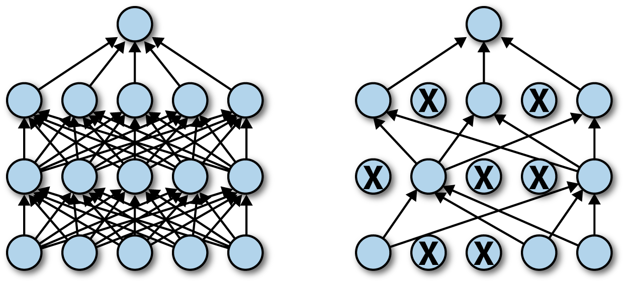
• By using a scale mixture Gaussian as a prior, noise parameters are removed while the valid signal is preserved, achieving both sparsity and expressiveness.

  \[\begin{aligned} P(\mathbf{w}) &=\pi \cdot \mathcal{N}(0,\sigma_{1}^{2}) + (1-\pi) \cdot \mathcal{N}(0,\sigma_{2}^{2}) \end{aligned}\]

• Reparameterization Trick is a technique that transforms the sampling process from an approximate distribution into a differentiable function:

  \[\begin{gathered} w_{i} \sim \mathcal{N}(\mu_{i},\sigma_{i}^{2})\\ \Downarrow\\ w_{i} = \mu_{i} + \sigma_{i} \cdot \epsilon_{i}, \quad \epsilon_{i} \sim \mathcal{N}(0,1) \end{gathered}\]

• Variational Inference:

  \[\begin{aligned} \text{ELBO} &= \mathbb{E}_{W \sim Q}\left[\log{P(\mathcal{D} \mid W)}\right] - KL[Q(W) \parallel P(W)] \end{aligned}\]