BPR

idea

• BPR(Bayesian Personalized Ranking): 관측 아이템과 미관측 아이템 간 로짓 격차를 최대화함으로써 AUROC(Area Under the Receiver Operating Characteristic) 최적화를 수행하는 학습 전략

  • 실제 서비스 환경에서 주로 제공되는 데이터 셋은 암시적 피드백이고, 추천시스템이 제공하여야 하는 서비스는 선호 여부 혹은 선호도를 정확히 맞추는 것이 아니라 다른 아이템들보다 선호할 가능성이 높은 아이템을 선별하여 제안하는 것임

  • 때문에 최적화는 개별 아이템에 대한 평점 혹은 선호 여부를 정확히 맞추는 것(조건부 우도를 최대화하는 것)이 아니라 선호할 가능성이 높은 아이템과 낮은 아이템의 예측 점수 격차를 최대화하는 것을 목표로 하여야 함(기수성이 아니라 서수성이 중요함)

auroc optimization

• roc is the set of $(x, y)$ pairs for all threshold $t$ values:

  \[\begin{aligned} \mathrm{roc} &=\left\{(x,y) \mid t \in [0,1]\right\} \end{aligned}\]

  • $x$ is FPR(False Positive Rate):

    \[\begin{aligned} x &=f(t)\\ &=p\left(\hat{z} > t\mid z=0\right) \end{aligned}\]

  • $y$ is TPR(True Positive Rate):

    \[\begin{aligned} y &=g(t)\\ &=p\left(\hat{z} > t\mid z=1\right) \end{aligned}\]

• auroc is the area under the roc curve:

  \[\begin{aligned} \mathrm{auroc} &=\int_{0}^{1}{g \circ f^{-1}\left(x\right)\mathrm{d}x} \end{aligned}\]

• $f(t), g(t)$ is related to cdf:

  \[\begin{aligned} f(t) &=p\left(\hat{z} > t\mid z=0\right)\\ &=1 - \underbrace{p\left(\hat{z} \le t\mid z=0\right)}_{\mathrm{cdf}}\\ \\ g(t) &= p\left(\hat{z} > t\mid z=1\right)\\ &= 1 - \underbrace{p\left(\hat{z} \le t\mid z=1\right)}_{\mathrm{cdf}} \end{aligned}\]

• change of variables:

  \[\begin{aligned} \frac{\mathrm{d}x}{\mathrm{d}t} &= \frac{\text{d}f(t)}{\mathrm{d}t}\\ &= -\underbrace{p\left(\hat{z}=t \mid z=0\right)}_{\mathrm{pdf}}\\ \\ \therefore \mathrm{d}x &= -p\left(\hat{z}=t \mid z=0\right)\mathrm{d}t \end{aligned}\]

• therefore:

  \[\begin{aligned} \mathrm{auroc} &=\int_{x=0}^{x=1}{g \circ f^{-1}\left(x\right)\mathrm{d}x}\\ &=\int_{t=1}^{t=0}{g(t) \frac{\mathrm{d}f(t)}{\mathrm{d}t} \mathrm{d}t}\\ &=-\int_{t=0}^{t=1}{g(t) \frac{\mathrm{d}f(t)}{\mathrm{d}t} \mathrm{d}t}\\ &=\int_{t=0}^{t=1}{p\left(\hat{z} > t\mid z=1\right) p\left(\hat{z}=t \mid z=0\right)\mathrm{d}t}\\ &=\int_{t=0}^{t=1}\int_{\tau>t}{p\left(\hat{z} = \tau\mid z=1\right) p\left(\hat{z}=t \mid z=0\right)\mathrm{d}t}\\ &=p(\hat{z}_{1} > \hat{z}_{0}) \end{aligned}\]

data set

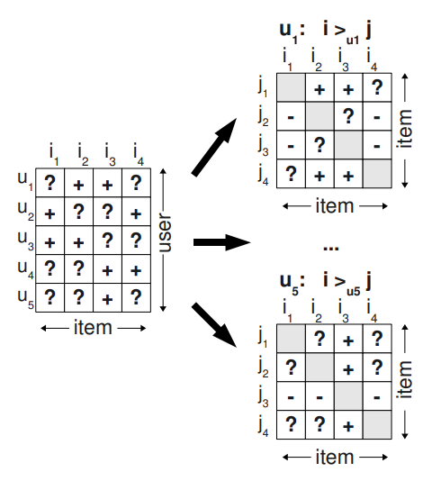
• 사용자 $u$ 의 선호체계 $>_{u}$ 에 관한 가정:

  • 비교 가능성(Totality):

    \[\forall i,j \in I:\quad i \ne j \quad \Rightarrow \quad \left(i >_{u} j\right) \vee \left(j >_{u} i\right)\]

  • 반대칭성(Anti-Symmetry):

    \[\forall i,j \in I:\quad \left(i >_{u} j\right) \wedge \left(j >_{u} i\right) \quad \Rightarrow \quad i = j\]

  • 이행성(Transitivity):

    \[\forall i,j,k \in I:\quad \left(i >_{u} j\right) \wedge \left(j >_{u} k\right) \quad \Rightarrow \quad \left(i >_{u} k\right)\]

• single data point definition:

  \[x_{u,i,j}:=\hat{y}_{u,i} - \hat{y}_{u,j}\]

• pair-wise data set:

  \[\Omega = \Big\{(u,i,j) \mid i \in I_{u} \wedge j \in I \setminus I_{u}\Big\}\]
  • $I$ : 아이템 집합
  • $I_{u} \subset I$ : 사용자 $u$ 가 관측한 아이템 집합
  • $i \in I_{u}$ : 사용자 $u$ 가 관측한 아이템
  • $j \in I \setminus I_{u}$ : 사용자 $u$ 가 관측하지 아니한 아이템

posterior estimation

\[\underbrace{\ln{P(\Theta \mid \mathcal{D})}}_{\begin{array}{c} \text{Objective Function} \\ \text{(Log Posterior)} \end{array}} \propto \underbrace{\ln{P(\mathcal{D} \mid \Theta)}}_{\text{Log Likelihood}} + \underbrace{\ln{P(\Theta)}}_{\text{Log Prior}}\]

• likelihood of single data point:

  \[\begin{aligned} P(i >_{u} j \mid \Theta) &=\sigma\left(\hat{x}_{u,i,j}\right) \end{aligned}\]

• likelihood of data set:

  \[\begin{aligned} P(\mathcal{D} \mid \Theta) &=\prod_{(u,i,j)\in\Omega}{P(i >_{u} j \mid \Theta)}\\ &=\prod_{(u,i,j)\in\Omega}{\sigma\left(\hat{x}_{u,i,j}\right)} \end{aligned}\]

• log likelihood:

  \[\begin{aligned} \ln{P(\mathcal{D} \mid \Theta)} &=\ln{\prod_{(u,i,j)\in\Omega}{P(i >_{u} j \mid \Theta)}}\\ &=\sum_{(u,i,j)\in\Omega}{\ln{P(i >_{u} j \mid \Theta)}}\\ &=\sum_{(u,i,j)\in\Omega}{\ln{\sigma\left(\hat{x}_{u,i,j}\right)}} \end{aligned}\]

• prior determination:

  \[\begin{aligned} \Theta &\sim \mathcal{N}\left(0, \lambda_{\Theta}^{-1}\mathbf{I}\right)\\ P\left(\Theta\right) &= \frac{1}{(2\pi)^{d/2} \cdot \lambda_{\Theta}^{d/2}} \cdot \exp \left[-\frac{\lambda_{\Theta}}{2}\Vert \Theta \Vert^{2}\right]\\ \\ \ln{P\left(\Theta\right)} &= \ln{\frac{1}{(2\pi)^{d/2} \cdot \lambda_{\Theta}^{d/2}} \cdot \exp \left[-\frac{\lambda_{\Theta}}{2}\Vert \Theta \Vert^{2}\right]}\\ &= \ln{\frac{1}{(2\pi)^{d/2} \cdot \lambda_{\Theta}^{d/2}}} - \frac{\lambda_{\Theta}}{2}\Vert \Theta \Vert^{2}\\ &\propto -\lambda_{\Theta}\Vert\Theta\Vert^{2} \end{aligned}\]

• posterior estimation:

  \[\begin{aligned} P(\Theta \mid \mathcal{D}) &\propto P(\mathcal{D} \mid \Theta) \cdot P(\Theta)\\ \\ \ln{P(\Theta \mid \mathcal{D})} &\propto \ln{P(\mathcal{D} \mid \Theta)} + \ln{P(\Theta)}\\ &\propto \sum_{(u,i,j)\in\Omega}{\ln{\sigma\left(\hat{x}_{u,i,j}\right)}} -\lambda_{\Theta}\Vert\Theta\Vert^{2} \end{aligned}\]

optimization

• objective function:

  \[\text{BPR-OPT} = \ln{P(\Theta \mid \mathcal{D})}\]

• optimization:

  \[\begin{aligned} \hat{\Theta} &= \text{arg} \max_{\Theta}{\ln{P(\Theta \mid \mathcal{D})}}\\ &= \text{arg} \max_{\Theta}{\sum_{(u,i,j)\in\Omega}{\ln{\sigma\left(\hat{x}_{u,i,j}\right)}} - \lambda_{\Theta}\Vert\Theta\Vert^{2}}\\ &= \text{arg} \min_{\Theta}{\sum_{(u,i,j)\in\Omega}{-\ln{\sigma\left(\hat{x}_{u,i,j}\right)}} + \lambda_{\Theta}\Vert\Theta\Vert^{2}} \end{aligned}\]
  • $\hat{\Theta}$ is MAP(Maximum a Posteriori) Estimator