Markov Chain Monte Carlo
Based on the lecture “Bayesian Modeling (2024-1)” by Prof. Yeo Jin Chung, Dept. of AI, Big Data & Management, College of Business Administration, Kookmin Univ.

Markov Chain Monte Carlo
-
마르코프 체인 몬테 카를로(
MarkovChainMonteCarlo) : 이전 단계에서 추출한 표본을 기반으로 다음 단계의 표본을 순차로 추출하여 사후 분포에 근사하는 방법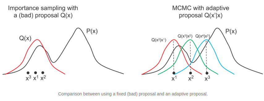
- Random-walk based MCMC
- Metropolis algorithm
- Metropolis–Hastings
- Random-Walk Metropolis
- Independence sampler
- Gibbs Sampling based MCMC
- Full Gibbs sampler
- Blocked Gibbs
- Collapsed Gibbs
- Gradient based MCMC
- Hamiltonian Monte Carlo
- No-U-Turn Sampler
- Riemannian Manifold HMC
Metropolis Hastings Method
-
메트로폴리스 헤이스팅스 방법(Metropolis Hastings Method) : 목표 분포의 산 모양을 추정하기 위하여, 확률 밀도가 높은 지역일수록(봉우리가 높은 지역일수록) 그 근방에서 더 많은 조약돌을 모으는 방법
-
inital sample:
\[\theta^{(t=0)}\] -
sampling candidate state $\psi$:
\[\psi \sim \mathcal{N}(\theta^{(t)},\sigma^2)\] -
conditional acceptance:
\[\theta^{(t+1)} =\begin{cases}\begin{aligned} \psi, \quad &\text{if} \quad u<\alpha(\theta^{(t)},\psi) \quad \text{for} \quad u \sim \text{Uniform}(0,1)\\ \theta^{(t)}, \quad &\text{otherwise} \end{aligned}\end{cases}\]
-
-
목표 분포(Target Dist.) : 파라미터 $\theta^{(t)}$ 의 사후 확률 분포
\[p(\theta^{(t)}\mid \mathcal{D}) \propto p(\theta^{(t)}) \cdot p(\mathcal{D} \mid \theta^{(t)})\] -
제안 분포(Proposal Dist.) : 시점 $t$ 에서 수락된 파라미터 샘플 $\theta^{(t)}$ 에 기반하여 다음 시점 $t+1$ 에서 샘플링 위치 $\psi$ 를 제안하는 분포
\[q(\psi \mid \theta^{(t)}) = \mathcal{N}(\theta^{(t)},\sigma^2)\]-
제안 분포가 $\theta^{(t)}$ 을 중심으로 하는 종형 분포인 경우:
\[q(\psi \mid \theta^{(t)}) = q(\theta^{(t)} \mid \psi)\] -
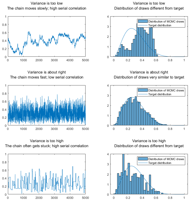
$\sigma^2$ 의 크기와 샘플링 수렴 여부의 관계:
-
-
수락 확률(Acceptance Prob.) : $\psi$ 를 다음 시점의 샘플 $\theta^{(t+1)}$ 로 수락할 확률
\[\begin{aligned} \alpha(\theta^{(t)}, \psi) &= \min{\left[1, \frac{p(\psi \mid \mathcal{D})}{p(\theta^{(t)} \mid \mathcal{D})} \cdot \frac{q(\theta^{(t)} \mid \psi)}{q(\psi \mid \theta^{(t)})}\right]}\\ &= \min{\left[1, \frac{p(\psi \mid \mathcal{D})}{p(\theta^{(t)} \mid \mathcal{D})}\right]} \quad \text{s.t.} \quad \psi \sim \mathcal{N}(\theta^{(t)},\sigma^2)\\ &\propto \min{\left[1, \frac{p(\psi) \cdot p(\mathcal{D} \mid \psi)}{p(\theta^{(t)}) \cdot p(\mathcal{D} \mid \theta^{(t)})}\right]} \end{aligned}\]
Auto-Correlation
-
자기상관(Auto-Correlation) : 순차로 발생한 일련의 관측치 ${x^{(t)} \mid t\text{ is time point}}$ 간에 존재하는 상관관계
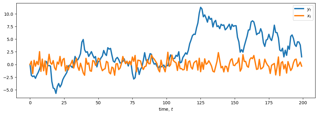
- $x^{(t)} \sim N(0,1) \quad \text{for} \quad x^{(0)} = 0$
- $y^{(t)} \sim N(y^{(t-1)},1) \quad \text{for} \quad y^{(0)} = 0$
-
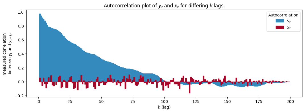
자기상관계수(Auto-Correlation Coefficient) : 순서에 의미가 있는 데이터에서, 현재 시점의 값 $x^{(t)}$ 과 그 과거 또는 미래의 값 $x^{(t-k)}$ 간의 상관관계를 측정하는 지표
\[R(k)=\text{Corr}(x^{(t)},x^{(t-k)})\]-
$k$ : 시간 간격(Lag)
-
-
솎아내기(Thinning) : 매 $k$ 번째 표본을 선택함으로써 자기상관을 줄이는 방법
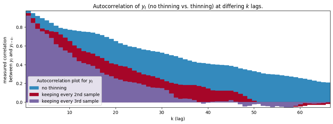
- 통상 $k \le 10$ 으로 설정함
-
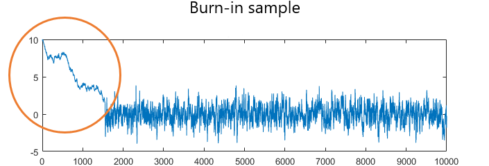
선행 구간(Burn-in Period) : 수렴 상태에 도달하기 전, 초기값 $x^{(t=0)}$ 의 영향력을 최소화하기 위해 일부 반복을 무시하는 구간
Evaluation Process: LOO
Metric
-
LPD(
\[\begin{aligned} \mathrm{LPD} &=\sum_{i=1}^{N}{\log{p(y_{i}\mid y_{\forall})}}\\ \underbrace{p(y_{i}\mid y_{\forall})}_{\text{posterior pred.}} &=\int{\underbrace{p(y_{i}\mid\theta)}_{\text{likelihood}}\underbrace{p(\theta\mid y_{\forall})}_{\text{posterior}}}{\mathrm{d}\theta} \end{aligned}\]LogPredictiveDensity): 훈련 시 학습한 관측치에 대한 적합도 -
ELPD(
\[\begin{aligned} \mathrm{ELPD} &=\sum_{i=1}^{N}{\log{p(y_{i}\mid y_{-i})}}\\ \underbrace{p(y_{i}\mid y_{-i})}_{\text{posterior pred.}} &=\int{\underbrace{p(y_{i}\mid\theta)}_{\text{likelihood}}\underbrace{p(\theta\mid y_{-i})}_{\text{posterior}}}{\mathrm{d}\theta} \end{aligned}\]ExpectedLogPredictiveDensity): 훈련 시 학습하지 않은 관측치에 대한 예측 성능 -
유효 파라미터 수(Effective
Parameter Count): 미관측 데이터 셋을 확인하였을 때 성능 개선폭으로서 과적합을 나타냄
\[\begin{aligned} p &=\mathrm{LPD}-\mathrm{ELPD} \end{aligned}\]파라미터 수 $K$ 가 훈련 관측치 수 $N$ 만큼 있다고 가정하자. 파라미터 하나당 관측치 하나를 직접 설명할 때 관측 데이터 셋 적합도가 최대가 될 것임. 이는 전체 모형이 일반화된 패턴을 전혀 포착하지 못하고 있는 과적합 상태가 됨. 따라서 모형의 적합도와 예측 성능 간 차이는 모형이 특정 관측치를 직접 맞추기 위해 실제로 사용한 자유도(복잡도)가 됨. 이는 모형이 데이터 셋에 적합되기 위해 추가 작동된(유효한) 파라미터 수로 해석할 수 있음.
Importance Sampling
-
Importance Sampling(IS): 기대값을 구할 때 목표 분포 $P$ 에서 확률변수 $\theta$ 를 샘플링하기 어려울 경우 근사 분포 $Q$ 에서 샘플링하되 Importance Weight 으로 가중하여 목표 분포 하의 기대값을 근사하는 방법
\[\begin{aligned} \mathbb{E}_{P(\theta)}\left[f(\theta)\right] &=\int{f(\theta)}{p(\theta)\mathrm{d}\theta}\\ &=\int{f(\theta)}{\frac{p(\theta)}{q(\theta)}q(\theta)\mathrm{d}\theta}\\ &=\int{\frac{p(\theta)}{q(\theta)}\cdot f(\theta)}{q(\theta)\mathrm{d}\theta}\\ &\approx\frac{1}{S}\sum_{s=1}^{S}{f(\theta^{(s)})\cdot\frac{p(\theta^{(s)})}{q(\theta^{(s)})}} \end{aligned}\] -
Importance Weight: 목표 분포 $P$ 와 근사 분포 $Q$ 의 비율로서, 샘플 $\theta$ 가 근사 분포 대비 목표 분포에서 얼마나 중요한지를 나타냄
\[\begin{aligned} w(\theta^{(s)}) &:=\frac{p(\theta^{(s)})}{q(\theta^{(s)})} \end{aligned}\]
Leave One Out Approximation
-
Leave One Out 에서 목표 분포는 관측치 $i=1,2,\cdots,N$ 마다의 사전 분포가 됨:
\[\begin{aligned} p(\theta\mid y_{-i}) \end{aligned}\] -
실제 계산된 분포는 전체 관측치의 사후 분포 하나임:
\[\begin{aligned} q(\theta) \approx p(\theta\mid y) \propto p(y_{i}\mid\theta)p(\theta\mid y_{-i}) \end{aligned}\] -
전체 관측치의 사후 분포를 활용하여 개별 관측치 $i$ 의 사전 분포들을 근사하는 경우 Importance Weight 는 다음과 같이 계산됨:
\[\begin{aligned} w_{i}(\theta^{(s)}) =\frac{p(\theta\mid y_{-i})}{p(\theta\mid y)} \propto\frac{1}{p(y_{i}\mid\theta)} \end{aligned}\] -
베이즈 정리에 따라 이는 우도의 역수가 됨. 즉, 샘플 $\theta^{(s)}$ 가 관측치 $y_{i}$ 를 잘 설명하지 못할수록 Importance Weight 가 커지며 이는 Importance Sampling 이 불안정함을 의미함:
\[\begin{aligned} \frac{p(\theta\mid y_{-i})}{p(\theta\mid y)} \propto\frac{\cancel{p(\theta\mid y_{-i})}}{p(y_{i}\mid\theta)\cancel{p(\theta\mid y_{-i})}} =\frac{1}{p(y_{i}\mid\theta)} \end{aligned}\]
Pareto k Diagnostic Plot
-
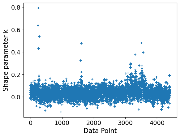
개별 관측치에 대하여 샘플 $\theta_{s}$ 에 대한 Importance Weight 의 분포를 생성한 후, 꼬리 부분만 선별하여 파레토 분포로 적합한다고 하자:
\[W\sim\mathrm{Pareto}(\beta,\alpha)\]- $\beta>0$: 척도 파라미터로서 확률변수 $W$ 가 취할 수 있는 최소값
- $\alpha>0$: 형상 파라미터로서 파레토 지수
-
파레토 지수가 $0$ 에 가까울수록 파레토 분포는 균등 분포에 근사하게 되고, 값이 클수록 디렉 델타 함수에 근사하게 됨:
\[\begin{aligned} \mathrm{Pr}(W>w) =\begin{cases} (\beta/w)^{\alpha},\quad &w\ge\beta\\ 1,\quad &w<\beta \end{cases} \end{aligned}\] -
파레토 지수의 역수 $k=1/\alpha$ 가 작을수록 특정 관측치를 설명하지 못하는 파라미터 샘플이 소수임을 의미함:
Probability Integral Transform
-
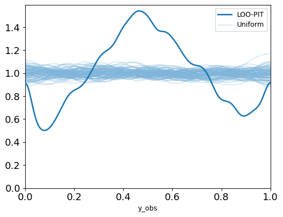
확률 적분 변환(
\[\begin{aligned} F(y_{i}) &=\mathrm{Pr}(y_{i}^{(\mathrm{rep})}\le y_{i}\mid y_{-i}), \quad y_{i}^{(\mathrm{rep})}\sim\mathcal{N}(\mu_{i},\sigma_{i}^{2}) \end{aligned}\]ProbabilityIntegralTransform): 관측값이 모형의 사후 예측 분포 안에서 어디쯤 위치하는지 측정하는 지표 -
확률변수 표준화:
\[z_{i} :=\frac{y_{i}-\mu_{i}}{\sigma_{i}}\sim\mathcal{N}(0,1^{2})\] -
누적 분포 함수 표준화:
\[F(y_{i})\longrightarrow\Phi\left(\frac{y_{i}-\mu_{i}}{\sigma_{i}}\right)\] -
표준 정규 분포의 누적 분포 함수값:
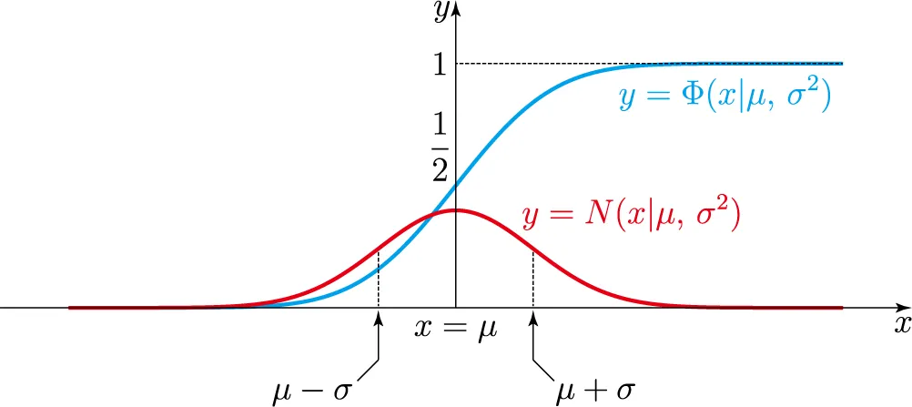
- $y=\mu\to\Phi(0)=0$
- $y>\mu\to\Phi\approx 1$
- $y<\mu\to\Phi\approx 0$
-
모형이 과신할수록($\sigma\downarrow$) 표준화된 관측값은 사후 예측 분포의 평균($0$)보다 극단적으로 크거나($\Phi\approx 1$) 극단적으로 작을 수 있어($\Phi\approx 0$) PIT 곡선이 $\cup$ 형태가 됨. 반대로 모형이 불확실성을 높게 잡을수록($\sigma\uparrow$) 표준화된 관측값은 사후 예측 분포의 평균($0$) 근처에 위치할 가능성이 높아($\Phi(0)=0$) PIT 곡선이 $\cap$ 형태가 됨:
PyMC Summary Indicator
-
Posterior Mean: 사후 평균 추정치
\[\hat{\mu}=\frac{1}{N}\sum_{i=1}^{N}{\theta_{i}}\] -
Posterior Standard Deviation: 사후 평균 추정치의 표준편차
\[\hat{\sigma}=\sqrt{\frac{1}{N-1}\sum_{i=1}^{N}{(\theta_{i}-\hat{\mu})^{2}}}\] -
\[\mathrm{MCSE}_{\mathrm{mean}} =\sqrt{\mathrm{Var}(\hat{\mu})}\approx \frac{\hat{\sigma}}{\sqrt{\mathrm{ESS}}}\]MonteCarloStandardError: 사후 평균 추정치의 몬테카를로 표준오차- Mean: 사후 분포의 중심 위치 추정 불확실성으로서 중심 위치 추정의 안정성
- Std: 사후 분포의 폭 추정 불확실성으로서 신뢰구간 추정의 정확성
-
\[\mathrm{ESS}=\frac{MN}{1+2\sum_{t=1}^{\infty}{\rho_{t}}}\]EffectiveSampleSize: 샘플 간 자기상관을 보정한 독립 샘플 수- Bulk: 중심부에서의 표본 독립성으로서 사후 분포의 중심 위치 통계량의 신뢰도
- Tail: 꼬리부에서의 표본 독립성으로서 신뢰구간 경계의 신뢰도
-
Gelman–Rubin Statistic (Potential Scale Reduction Factor): 체인 간 수렴성 평가 지표
\[\hat{R}=\sqrt{\frac{B}{W}}\]-
Definition:
\[\begin{aligned} \bar{\theta}^{(k)}:=\frac{1}{N}\sum_{i=1}^{N}{\theta_{i}^{(k)}}, \quad \bar{\theta}:=\frac{1}{M}\sum_{k=1}^{M}{\bar{\theta}_{k}} \end{aligned}\] -
Between-chain variance:
\[\begin{aligned} B=\frac{N}{M-1}\sum_{k=1}^{M}{(\bar{\theta}^{(k)} - \bar{\theta})^{2}} \end{aligned}\] -
Within-chain variance:
\[\begin{aligned} W&=\frac{1}{M}\sum_{k=1}^{M}{s_{k}^{2}}\\ s_{k}^{2}&=\frac{1}{N-1}\sum_{i=1}^{N}{(\theta_{i}^{(k)}-\bar{\theta}^{(k)})^{2}} \end{aligned}\]
-
Source
- https://www.statlect.com/fundamentals-of-statistics/Markov-Chain-Monte-Carlo