t-SNE

Prerequisite

---

• 정보이론(Information Theory): 신호에 존재하는 정보의 양을 측정하는 이론으로서, 특정 확률분포의 특성을 알아내거나, 두 확률분포 간 유사성을 정량화하는 데 사용함

• Shannon’s Information Theory Principles
  • 자주 발생하지 않는 사건(Unlikely Event)일수록 높은 정보량을 가짐(Informative)
    • 해가 동쪽에서 뜨는 사건은 사람들이 확신하고 있는 사건이므로 정보량이 낮은 반면, 해가 서쪽에서 뜨는 사건은 자연 법칙을 거스르는 극히 드문 사건이므로 정보량이 높음
  • 독립사건은 추가적인 정보량을 가짐(Addictive Information)
    • 동전을 두 번 던져서 앞면이 두 번 나오는 사건은 동전을 한 번 던져서 앞면이 나오는 사건보다 정보량이 두 배임

• 자기정보(Self-Information): 확률변수 $X \sim P$ 에 대하여, 사건 $X=x$ 가 발생했을 때의 정보량

  \[\begin{aligned} I(X=x) &=-\log{P(X=x)} \end{aligned}\]

• 엔트로피(Entropy): 자기정보의 기대값으로서, 주어진 확률분포에서 발생 가능한 사건들의 평균적인 정보량

  \[\begin{aligned} H(P) = \mathbb{E}_{X \sim P}\left[I(X)\right] = -\sum_{X}{\log{P(x)} \cdot P(x)} \end{aligned}\]
  • 사건의 분포가 결정적일수록(Deterministic) 엔트로피가 감소함
  • 사건의 분포가 균등할수록(Uniform) 엔트로피가 증가함

• 교차 엔트로피(Cross Entropy): 확률변수 $X$ 의 분포 $P$ 와 그 근사 분포 $Q$ 에 대하여, $Q$ 가 $P$ 에 대하여 제공하는 정보의 불확실성을 측정하는 지표

  \[\begin{aligned} H(P,Q) = \mathbb{E}_{X \sim P}\left[-\log{Q(X)}\right] = -\sum_{X}{\log{Q(X)} \cdot \log{P(X)}} \end{aligned}\]

• 쿨백 라이블러 발산(Kullback-Leibler Divergence): 확률변수 $X$ 의 분포 $P$ 와 그 근사 분포 $Q$ 에 대하여, $Q$ 를 $P$ 의 근사 분포로 사용할 때의 비효율성을 측정하는 지표로서, $P$ 에서 샘플링된 $X$ 에 대하여, $P$ 가 제공하는 평균적인 정보량과 $Q$ 가 제공하는 평균적인 정보량의 차이

  \[\begin{aligned} KL[P(X) \parallel Q(X)] = H(P,Q) - H(P) = \sum_{X}{\log{\frac{P(X)}{Q(X)}} \cdot P(X)} \end{aligned}\]

t-SNE

---

• t-분포 확률적 이웃 임베딩(t-Distribution Stochastic Neighbor Embedding): 고차원 공간 상에서의 관측치 간 거리를 보존하면서 관측치 간 고차원 공간 상 확률적 유사도를 보존하면서 저차원으로 매핑하는 비선형 차원 축소 기법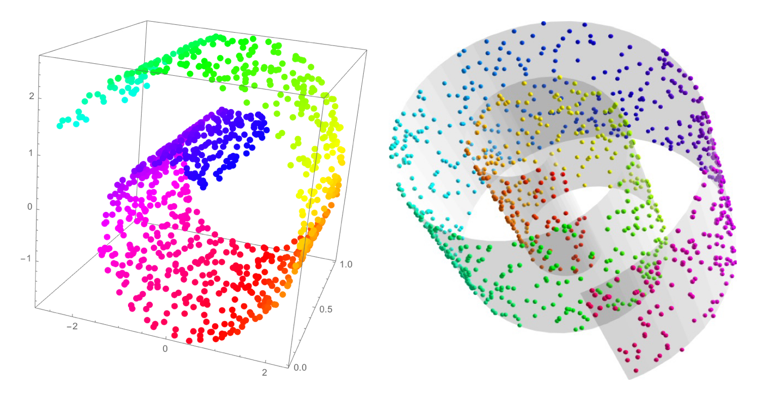

  

Similarity Dist. in High Rank

• Gaussian Kernel:

  \[\begin{aligned} \mathcal{K}(\overrightarrow{\mathbf{x}}_{i}, \overrightarrow{\mathbf{x}}_{j}) &= \exp{\left[-\frac{\Vert \overrightarrow{\mathbf{x}}_{i}-\overrightarrow{\mathbf{x}}_{j}\Vert^{2}}{2\sigma_{i}^{2}}\right]} \end{aligned}\]

• Gaussian-based Conditional Probabilities:

  \[\begin{aligned} p(j \mid i) &= \frac{\mathcal{K}(\overrightarrow{\mathbf{x}}_{i}, \overrightarrow{\mathbf{x}}_{j})}{\sum_{k \ne i}{\mathcal{K}(\overrightarrow{\mathbf{x}}_{i}, \overrightarrow{\mathbf{x}}_{k})}} \end{aligned}\]

• Symmetrization of probability through joint probability calculation:

  \[\begin{aligned} p(i,j) &= \frac{p(j \mid i) + p(i \mid j)}{2n} \end{aligned}\]

Similarity Dist. in Low Rank

• Cauchy Dist. Kernel:

  \[\begin{aligned} \mathcal{K}(\overrightarrow{\mathbf{y}}_{i}, \overrightarrow{\mathbf{y}}_{j}) &= \frac{1}{1 + \Vert \overrightarrow{\mathbf{y}}_{i} - \overrightarrow{\mathbf{y}}_{j} \Vert^{2}} \end{aligned}\]
  • cauchy dist. is t-dist. when the degree of freedom is $1$

• L1 Regularization:

  \[\begin{aligned} q(i,j) &= \frac{\mathcal{K}(\overrightarrow{\mathbf{y}}_{i}, \overrightarrow{\mathbf{y}}_{j})}{\sum_{k \ne l}{\mathcal{K}(\overrightarrow{\mathbf{y}}_{k}, \overrightarrow{\mathbf{y}}_{l})}} \end{aligned}\]

Optimization

• Objective Function:

  \[\begin{aligned} \mathcal{L} &=\sum_{i}{KL[P(i) \parallel Q(i)]}\\ &= \sum_{i}\sum_{j}{\log{\frac{p(i,j)}{q(i,j)}} \cdot p(i,j)} \end{aligned}\]

• Optimization:

  \[\begin{aligned} \hat{\mathbf{Y}} &= \left\{\overrightarrow{\mathbf{y}}_{i} \mid \text{arg} \min{\mathcal{L}}\right\} \end{aligned}\]